Using the Litz Wire Feature in CST Studio Suite

Introduction

The use of litz wires as conductor windings in low frequency (LF) applications is growing due to its multiple benefits of carrying alternating current (AC) at high frequencies, up to the MHz range, where skin and proximity effects in a solid conductor become a significant problem. Litz wire conductors are made of multiple strands of insulated copper wire woven/twisted together in an optimized manner so that the flowing current is homogeneous and the losses are mitigated. In LF, litz wires are predominantly used in transformers and inductors. Their use is now being extended to a wider range of applications, such as windings in electrical machines and coils in general.

Modeling litz wires is important so that the losses due to skin and proximity effects can be calculated to the required level of accuracy. However, it can be very onerous in terms of geometry modeling and simulation time to represent each strand in the litz wire conductor, hence the need for an alternative method. In CST Studio Suite, an effective wire approach is used to represent the strands of the conductor, shortening modeling and simulation times.

In this paper, we focus on the simulation of litz wires with the CST Studio Suite LF solver, where we added a feature to simplify the modeling. We demonstrate litz wire results with an example.

Physical Effects within Litz Wires

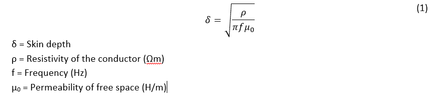
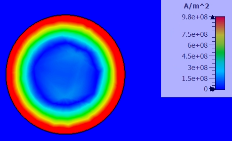
When an alternating current flows at high frequencies in a solid wire, there is a redistribution of the current within the conductor. The current density is largest near the outer surface of the conductor and decreases exponentially toward the inner axis of the conductor. This redistribution is the skin effect. The expression for the skin depth δ is given in (1) and its effect is shown in Figure 1. The outer red cross-section in Figure 1 carries the highest current magnitude while the central blue section carries the lowest current magnitude, which is due to redistribution of current flow inside the whole cross-section of the conductor. The skin depth, δ, is therefore the depth where the current density is 1/e of the value at the surface.

This causes an increase in resistance of the conductor due to reduced cross-sectional area of current flow, and therefore resulting in an increase in heat losses. Using litz wires in such cases helps mitigate the skin effects but does not eliminate it; hence why it must be taken into account.

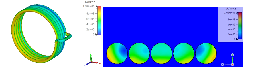
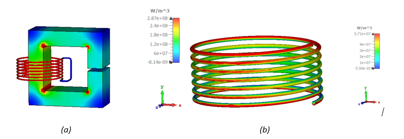
Another significant issue to consider when using litz wires is the proximity effect due to the closeness of packed wires. The proximity effect also causes a redistribution of currents within the conductors and hence an increase in AC resistance, resulting in an increase in heat losses. Figure 2 shows how the proximity effect affects current distribution in a coil with five turns. Figure 2 (a) shows the full coil, and Figure 2(b) the current distribution in the cross section. Twisting the wire strands into a bundle using an appropriate lay length and number of twists can help reduce the losses due to the proximity effect, but does not eliminate them. Hence, we must also consider them.

Modeling Litz Wires in CST Studio Suite

The losses discussed earlier can be calculated in CST Studio Suite by effectively modeling the litz wires. We have added a new feature to allow the user to obtain a good approximation of the skin and proximity losses without having to model each strand of the litz wire.

The conductor can be modeled using the Coil features in CST Studio Suite, such as Coil Segment, where a cross-sectional profile and an open path are used to create the open coil segment. This feature will be extended to closed loop coils in future releases.

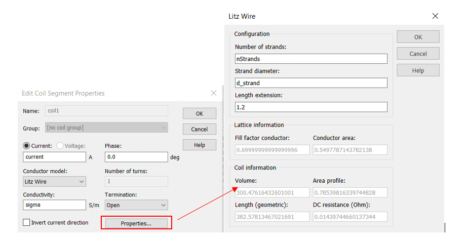
This feature allows you to set various parameters of the litz wire, like current, electrical conductivity, number of strands, strand diameter and the length extension factor of the wire (considering twisting and weaving length of strands). Other parameters relating to the geometry of the modeled coil are calculated automatically using the geometric dimensions of the coil and the parameters listed earlier. These include fill factor, (effective) conductor area, volume of coil, area of coil cross section, geometric length of coil and DC resistance.

Once the model is correctly set up, it must be solved using the LF Frequency Domain MQS Solver in CST Studio Suite. The frequencies of interest are set up for the model at which the losses are calculated.

Example Setup

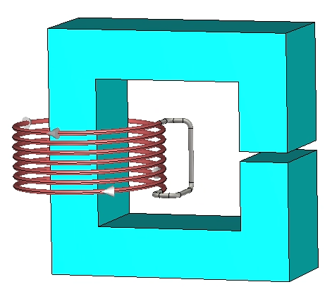
In this section, a simple example of a litz wire conductor wrapped on the leg of a ferrite C-core is used, as shown in Figure 3.

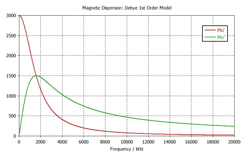
The relative magnetic permeability of the ferrite core is set to 200, and it has dispersive magnetic properties, as shown in Figure 4. This allows the calculation of the frequency-dependent magnetic losses in the C-core, which are not discussed in more detail here as it is beyond the scope of this paper.

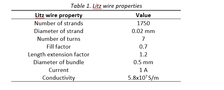
The coil is defined using ‘Coil Segment’ option and hence is by default an open coil loop. To have a divergence-free current in the coil, it must be closed either using a perfect electric conductor (PEC) or using the boundaries of the model. In this case, PEC is used as material to close the loop, as shown in Figure 3. This does not affect the losses in the model, but the PEC material can later be changed to a more realistic one to represent the electrical connector between the two wire ends. Once the coil is created, the properties can be defined in the dialog box, as shown in Figure 5. Table 1 provides more details on the litz wire coil used in this example.

The current amplitude specified here can be either RMS or peak values, depending on what is chosen in the solver window.

In general, the number of strands found in a litz conductor can range from a dozen to thousands. The strand diameter must be given without the insulation thickness and the software calculates the fill factor and conductor area, based on the cross-sectional area of the geometry of the coil. Usually, the maximum strand diameter chosen is twice the skin depth of the wire material used at the highest operating frequency. However, this is not always enough to eliminate skin losses, as real power supplies usually contain higher noise harmonics, depending on the application. The length extension is the ratio of the real total length of the litz wire (before twisting) to the measured final length (after twisting). This method assumes that the current is homogeneous at bundle level. Most industrially wound Litz wires have the strands twisted and woven in an optimized way to have the current as homogeneous as possible.

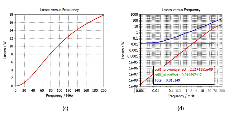
The model is solved for a frequency range of 50 Hz to 200 MHz, and the results for each frequency point can be found in the navigation tree, as shown in Figure 6(a). The main results of interest, skin and proximity losses, can be found under 1D Results/LF Solver/Losses. In this example, the losses in the ferrite C-core are also available. Figure 6(b), 6(c) and 6(d) show the skin, proximity and total losses respectively.

In Figure 6(b), we see the skin losses are relatively constant throughout the frequency range, except for the slight dip around 100 MHz. The relatively constant value is expected as the strand diameter is chosen (Table 1) below 2δ (two times the skin depth) up until a frequency of 100 MHz.

In Figure 6(c), we see an increase in proximity losses with increasing frequency, as expected. The magnitude of the proximity losses is large compared to the skin effect, as expected due to the diameter of strands chosen.

Figure 6(d) shows the total losses, including the ferrite C-core losses in logarithmic scale so that the values for the whole broadband range are visible. The legend shows the value of each loss at 50 Hz, which is the lowest simulated frequency. The slope is dominated by the ferrite losses, but the effect of the AC current losses is still significant, especially the proximity losses.

Figure 7(a) shows the magnetic loss density in the complete model at 100 MHz, while Figure 7(b) shows the loss density in the coils only, dominated mostly by the proximity effects. Despite the losses being much higher in the ferrite core, the loss density is much higher in the coils due to the smaller cross-sectional area.

•                                                                                         (b)

Losses Comparison in Non-Litz Wire Coils

If an evaluation without the litz wires was done on the same model in CST Studio Suite using Coil Segment, it would not be reasonable to compare the losses as the skin and proximity effects for a similar size wire conductor would not be taken into account. The software would only calculate the ohmic DC losses of the conductor and hence not provide a like-for-like comparison. This would also suggest that the AC losses in the non-litz wire conductor are smaller than with litz wires, which would be incorrect.

Conclusion

Litz wires are gaining popularity in the higher frequency spectrum of low frequency (LF) AC applications to reduce power loss. This paper has given a succinct overview of the new litz wire feature in CST Studio Suite, aiming to calculate skin and proximity losses more effectively, which become significant with higher frequencies. The types of losses arising in those applications are outlined, and a simple example of setting up a model with litz wires in CST Studio Suite is presented. The results are discussed, demonstrating the importance of calculating AC losses in conductors.

Interested in the latest in simulation? Looking for advice and best practices? Want to discuss simulation with fellow users and Dassault Systèmes experts? The SIMULIA Community is the place to find the latest resources for SIMULIA software and to collaborate with other users. The key that unlocks the door of innovative thinking and knowledge building, the SIMULIA Community provides you with the tools you need to expand your knowledge, whenever and wherever.