
In this blog post I would like to show how SIMULIA true transient EM/circuit co-simulation can be used to design reliable backplanes. I will show how KPIs and figures of merit such as the eye diagram can be calculated in simulation without having to test a physical prototype, and demonstrate the benefit of transient co-simulation (tran-co) over a macromodel circuit simulation method.
Introduction to backplanes modeling with IBIS-AMI
Design of long reach backplanes is a challenging task. Typically the data rate is up to tens of gigabauds and the channel length is about 1 meter. Traditional dielectrics like FR4 with loss tangent = 0.02 will lead to significant insertion loss (IL) on such a long channel. New materials with lower loss are necessary to mitigate IL. Line impedances at transmitters, receivers and connectors should match to achieve low return loss (RL).
Input/output Buffer Information Specification (IBIS) [1] is widely accepted in the industry for the modeling of input/output (I/O) buffers. IBIS Algorithmic Modeling Interface (IBIS-AMI) [1] allows vendor specific equalizations and clock recovery algorithms, which are mandatory parts of a Serializer/Deserializer (SerDes) PHY. The first step of AMI simulations is to obtain the impulse response of the passive channel and I/O buffer models, which is equal to the derivative of the step response.
True transient EM/circuit co-simulation
In the traditional workflow, the scattering parameter (S-Parameter) of the passive channel is calculated first and then converted to a SPICE model via standard macromodeling. In the end, the step response is obtained by simulating the SPICE model.
In comparison to the traditional workflow, a new transient EM/circuit co-simulation (tran-co) method [2] is introduced to calculate the step response without using S-parameters and macromodels, which solves Maxwell’s equations and circuit elements (e.g. IBIS models or AC coupling capacitors) together in time domain. It turns out to be faster than the traditional workflow and can also avoid nonphysical behaviors.
Insertion loss on a backplanes passive channel
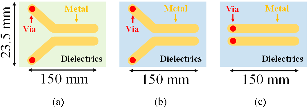
Before designing a 1-meter-long passive channel, three shorter test boards are investigated. Test board A: dielectrics with loss tangent = 0.02 and permittivity = 4.2 and mismatched impedance; Test board B: dielectrics with loss tangent = 0.008 and permittivity = 3.2 and mismatched impedance; Test board C: dielectrics with loss tangent = 0.008 and permittivity = 3.2 and matched differential impedance of 100 ohm at transmitter and receiver.
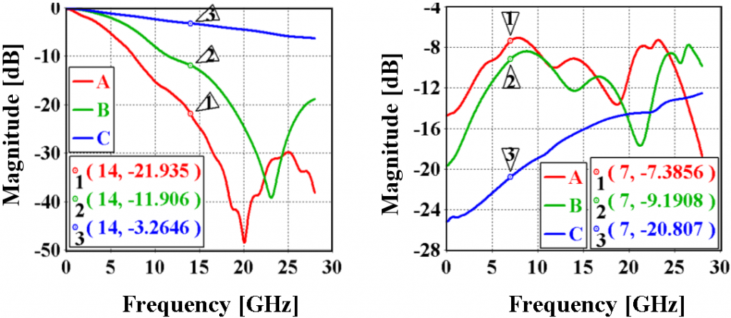
The simulation results are summarized in the following figure. By comparing SDD21 of curve A and B in the following left figure, we can observe the effect of dielectric loss on the insertion loss. For a 1-meter-long channel, typical dielectrics like FR4 with loss tangent = 0.02 will result in significant insertion loss, which already drops to -12 dB for the 150 mm channel. So new materials with lower loss are preferred. Comparing SDD11 curves of B and C in the right figure shows that it is important to keep the impedance matched especially at vias and connectors, where the cross section of differential pairs may change significantly.
Macromodel of SerDes step response
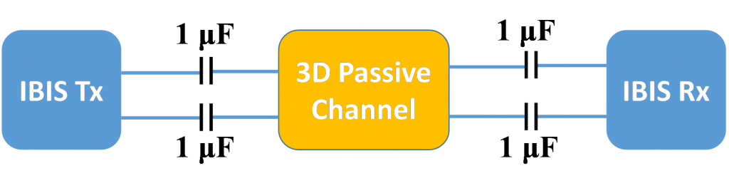
In the following, we calculate the step response of the SerDes channel, which contains IBIS Tx/Rx buffer models, AC coupling capacitors and 3D passive channel.
S-parameters of the 3D passive channel are calculated first and then converted to a macromodel, which can be simulated together with circuit elements (i.e. IBIS models and AC coupling capacitors) in the time domain to obtain the step response. In this blog this workflow is referred to as traditional or circuit workflow. However for a long passive channel (e.g. tens of λ, with free space wavelength of the maximum simulation frequency λ), S-parameter calculation could be time consuming and the standard macromodeling process might lead to inefficiencies (due to the large size of the final circuit) and accuracy degradation in the system level simulation (due to an inaccurate modeling of the propagation delay). For this reason, we introduce the tran-co workflow [2], which doesn’t need calculate S-parameter or macromodels and solves the 3D passive channel and circuit elements step by step together in the time domain to obtain the step response. We apply circuit and the tran-co workflow to the test board C and summarize their performance in the following table.
Table Ⅰ. Simulation statistics of Test board C
Max. Freq. Board Length Mesh Cells Circuit Tran-co
112 GHz 150 mm ≈ 56 λ 68,186,250 117 min 86 min
As shown in the table above, the tran-co workflow is faster than the circuit workflow. Simulations are run on a machine with a CPU @2.0 GHz, a GPU 2xKepler Tesla K40c+m and 256 GB RAM.
Comparing transient co-simulation and macromodel circuit simulation
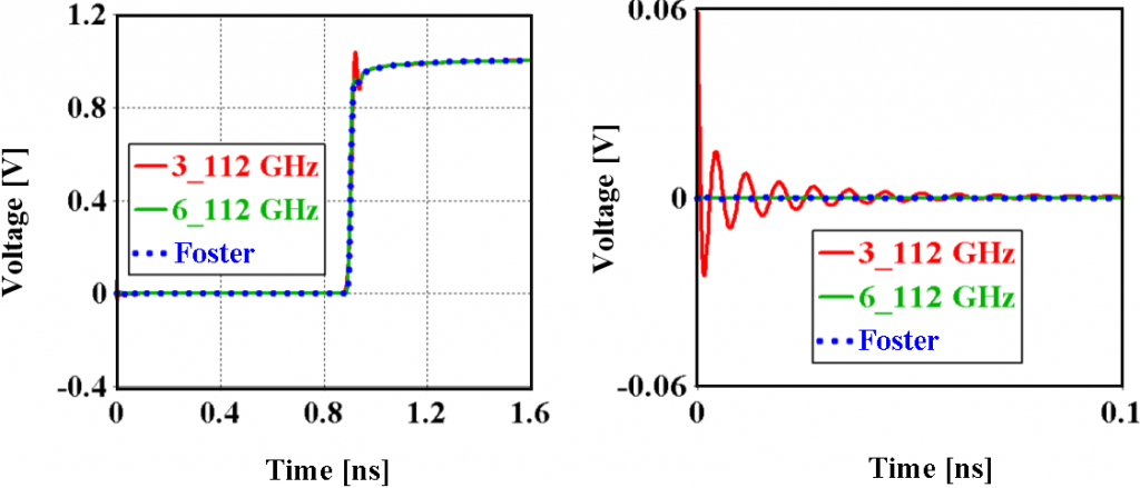
The step response of the tran-co workflow is compared to the results obtained by simulating a macromodel synthesized by using a residues-poles form (Foster Pole-Residue [2]) in a circuit solver [3]. As shown in the following, when using a macromodel synthesized as lumped elements, nonphysical ripples appear at the beginning of the step response (red, 3_112 GHz). But results of the tran-co workflow (green, 6_112 GHz) and poles/residues-based macromodel in the circuit workflow (blue, Foster) match each other and can avoid the nonphysical behaviors.
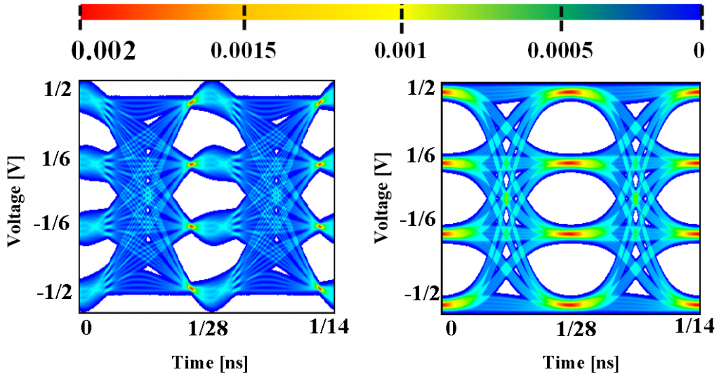
Statistical eye diagrams are generated for the circuit and tran-co workflows. It can be observed that the eye diagram of the circuit workflow with a macromodel synthesized as lumped elements is deformed as shown in the left figure below. The right figure below is the eye diagram for the tran-co workflow.
Full 3D backplanes channel simulation
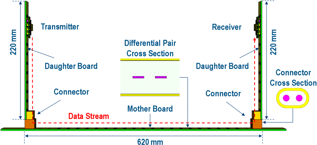
Finally we follow the tran-co workflow to simulate a 1-meter-long channel on the backplane as shown in the following figure. The differential impedance of the transmission line and connectors are optimized to 100 ohm. Loss free dielectrics with permittivity = 3.2 are used for the substrate.
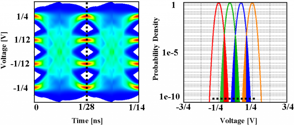
After obtaining the step response, 3-taps-FFE (Feedforward Equalizer) with 1 pre- and 2 post taps and 3-taps-DFE (Decision Feedback Equalizer) are used to improve the statistical eye diagram, which does not include random jitter. So the probability density (PD) of each level contains deterministic jitter only. We convolve the deterministic jitter of the eye diagram with a random noise and obtain the PD with a signal-to-noise ratio (SNR) of 12dB as shown below.
Backplane simulation workflow overview
SIMULIA CST solutions for SerDes simulation are summarized in the following picture.
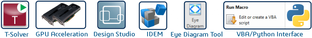
CST Studio Suite® Time Domain Solver [2] with GPU acceleration can simulate electrical large passive interconnects in the SerDes channel efficiently. IBIS-AMI [1] and HSPICE [3] simulation can be run in CST Design StudioTM. In the version 2022, an IBIS-AMI demo will be added in the component library, so that the users can get start with the IBIS-AMI simulation smoothly. CST Studio Suite® IDEM [2] provides state-of-the-art macromodeling techniques, which convert S-parameters to SPICE models. With the Eye Diagram Tool, users can also apply common SerDes techniques (e.g. equalization, or four-level pulse amplitude modulation (PAM4)) to their passive channel designs. The Eye Diagram Tool supports user defined Random Jitter (RJ) and statistical eye diagram. Last but not least, simulation results (e.g. differential S-parameters or probability density function) can be easily accessed by the VBA Macro Editor in CST and Python. So users can perform further analysis with VBA and Python scripts, like Channel Operating Margin (COM) [4], Error Propagation (EP) and Forward Error Correction (FEC), which are not supported by the IBIS-AMI Standard [1].
References
- IBIS Open Forum, https://ibis.org/.
- Dassault Systèmes, https://www.3ds.com/simulia/.
- Synopsys Inc. https://www.synopsys.com/.
- IEEE Std. 802.3bj-2014.
SIMULIA offers an advanced simulation product portfolio, including Abaqus, Isight, fe-safe, Tosca, Simpoe-Mold, SIMPACK, CST Studio Suite, XFlow, PowerFLOW and more. The SIMULIA Community is the place to find the latest resources for SIMULIA software and to collaborate with other users. The key that unlocks the door of innovative thinking and knowledge building, the SIMULIA Community provides you with the tools you need to expand your knowledge, whenever and wherever.

Longfei Bai joined SIMULIA CST, Dassault Systèmes in 2015 as an application engineer supporting customers with EDA. He completed his B.S. from the University of Electronic Science and Technology of China in 2011 and M.S. degrees from Technische Universität Darmstadt in 2015 in the field of electrotechnics. His primary focus now is on SI, PI and EMC on PCB, package and chip.