Performance Assessment of a Peristaltic Pump

The following is an excerpt of a blog post about a peristaltic pump that originally appeared on the SIMULEON blog and is written by Nikolaos Mavrodontis. To read the post in it’s entirety, visit the SIMULEON site, here. 

---

In this blog post, we will be showcasing a fully coupled fluid structure interaction (FSI) analysis, of a peristaltic roller pump. This study will focus on assessing the performance of a peristaltic pump, under operation. This co-simulation analysis, will solve for both the structural and fluid domains’ unknown quantities, during 1 revolution of the rotating mechanism of the pump.

This is an example of a challenging application, in which numerical modelling and computer simulations can provide a lot of insight and value.

The aspects we want to evaluate in this digital model are; determining the volume flow-rate for a given rotation speed, assessing contact stress areas on the tube, and determining the torque output for the given rpm.

Introduction

Peristaltic pumps are positive displacement pumps used extensively in many engineering disciplines, for transporting highly viscous fluids, or fluids with suspended solids.

The blog post’s peristaltic pump geometry and included components are given in Figure 1.

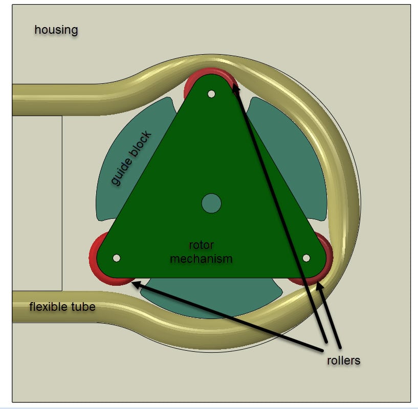
Figure 1: 3 roller peristaltic pump geometry

Study focus

The focus of this simulation study will be to assess the performance of the peristaltic pump. Based on the available output, different aspects of the peristaltic pump can be evaluated. Mainly:

• inspection of pressure/velocity fields for a certain rotor speed(rpm)  and volume flow rate Q(lt/min) .This can provide insight on the overall performance and rating of the pump
• inspection of structural stresses/strains on the flexible tube due to roller action and fluid pressures. This can quickly help determine potential failure locations, in case the tube is overstressed. Additionally stress output can be used for assessing the fatigue life of the flexible tube.
• inspection of contact stresses (contact pressure and shear). This can help improve the design of the roller geometry and rotor design.
• Torque output can be used for assessing the rotor’s performance for different flow rates or rotor speeds
• Velocity vectors can provide insight on the optimum surface characteristics that the flexible tube must have, to deliver a specific flow rate. This becomes particularly important when the pump transports highly viscous fluids, as lower flow rates are typically delivered in such cases.

Working principle of peristaltic pump

The pump (Figure 1) comprises of a housing, that encloses the rest of the pump’s components. A flexible tube that will contain the fluid, is held in place against the surrounding components. A rotor, that is fitted with three rollers, rotates in a predefined manner. These rotating rollers, occlude (block)  the tube, creating a temporary seal between the suction (fluid inlet) and discharge (fluid outlet) sides. As the rotor turns, the sealed pressure segments( the “pillows” of fluid), will move along the tube, forcing the product into the discharge outlet. Where the sealed pressure segments open up,  pressure is recovered, which acts as suction, drawing more fluid into the suction side of the pump.

The working principle for this type of pump, relies on  peristalsis. The human body as well, relies greatly on peristaltic processes. The human gastrointestinal tract and esophagus are two examples of such processes. In the human esophagus, radial contractions and relaxations of soft muscles, advance the food towards the stomach while preventing it from being pushed back into the mouth.  An impression of peristalsis is given in Figure 2.

Figure 2: peristalsis (image rights-Wikipedia)

Highlights of peristaltic pumps

• Can pump a large variety of challenging fluids
• Due to the gentle pumping action of the peristaltic pump, shear-sensitive polymers or even food products can be transferred
• The components of the peristaltic pump, are relatively simple, and robust, which means that those pumps are reliable and down time or maintenance is quite limited.
• The  flow rate of a peristaltic pump is proportional to the rotor speed, which means that peristaltic pumps are well suited for dosing (e.g. medical sciences but not only).
• There is a wide variety of available  materials for the flexible tube, making peristaltic pumps appealing for pumping highly corrosive or high temperature fluids
• As peristaltic pumps are enclosed in a casing and typically do not include seals, at the event of a tube rupture, the fluid remains contained, not allowing for cross contamination.
• Peristaltic pumps do not require priming. There is no requirement for continuous fluid flow at the pump’s inlet. Air or offgas being present within the flexible tube, are also pumped together with the fluid. The presence of air in the pump, can affect the pump’s performance, however.
• Cavitation is not an issue with peristaltic pumps

Computer models

Structural Model Abaqus

Geometry

A detail of the mesh of the pump assembly in Abaqus, is given in Figure 3. The color code in Figure 3, represents the distinction between rigid and deformable bodies, for the co-simulation.

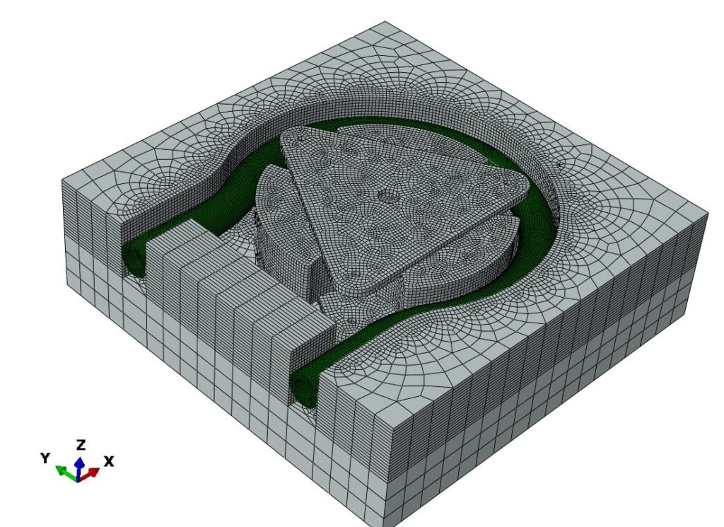
Figure 3: Mesh and body attributes (green=deformable/grey=rigid body) of peristaltic pump assembly in Abaqus

In particular, the grey colored components (housing, guide block, rotor mechanism) were modelled as rigid bodies, in order to reduce computational times. The dark green flexible tube was modelled as a deformable body, as this was the main focus for this analysis. The roller instances are not present in Figure 3. This is due to modelling convenience and is explained in Loads and BCs, below.

Material Modeling

For the rubber flexible tube in Abaqus, a hyperelastic material law (Ogden, 3rd order/ρ=1400 kg/m3) was used.

Contact interactions

Several contact interactions were set up for the finite element model. For the included contact interactions,  friction (μ=0.25) was used. Contact pairs were created for interaction between:

• pump housing to flexible tube
• guide block to flexible tube
• 3 pump rollers to flexible tube

Figure 4, shows a detail of the coupling surface, which will allow for information exchange between the stuctural and computational fluid dynamics solver.

This coupling surface will be the flexible tube’s wetted interior surface, which will be in contact with the fluid. A respectful interaction (Int-1 Fluid-structure Co-Simulation boundary) needs to be set up in Abaqus for this purpose, as it is shown below.

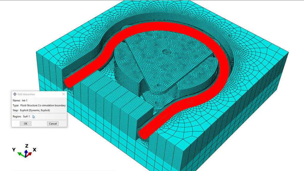
Figure 4: Fluid structure co-simulation boundary interaction/Flexible tube’s surface wetted by the fluid domain.

Loads and BCs

In terms of Boundary conditions,only the flexible tube end faces were fully fixed. The rigid bodies in the analysis were either fully constrained (e.g. housing), or assigned appropriate boundary conditions (guide block, rollers) to allow for a clockwise rotation. The rollers were also free to rotate around their own axis, additional to the motion prescribed to the rotor.

The initial relative positioning of the rollers-tube was different than in Figure 1. Specifically, it was more convenient to initially position the rollers at the center of the pump head(t=0), and then displace them to their final configuration, prior to the rotation of the pump head(t=0.1 sec). In this configuration, two rollers occluded the flexible tube, creating the first pillow of fluid for the analysis. This is shown in Figure 5 below.

Figure 5: roller configuration at t=0 sec (left) and prior to pump head rotation, at t=0.1 sec (right)

The configuration of the rollers-tube at t=0.1 sec could have also been achieved, with interference fit instead.

No gravity load was applied.

Step settings

An Abaqus explicit step was used for the co-simulation example. The analysis time was equal to 1.1. sec. The same analysis time was used in the CFD solver. The analysis time allowed for one revolution of the rotor, essentially modelling a roller pump with a 60 rpm (revolution per minute) rotor speed.

CFD model XFlow

Geometry and initial conditions

The geometry of the CFD model only contains the flexible tube geometry. This is the component in which fluid will flow and also contains the wetted surface that will be used for the coupling between Abaqus-Xflow (see Figure 4).

Additionally, basic inlet/outlet conditions have been set up in the Xflow model. Gauge pressures (0 Pa at inlet) were used for the cfd model. A detail is given in Figure 6 below.

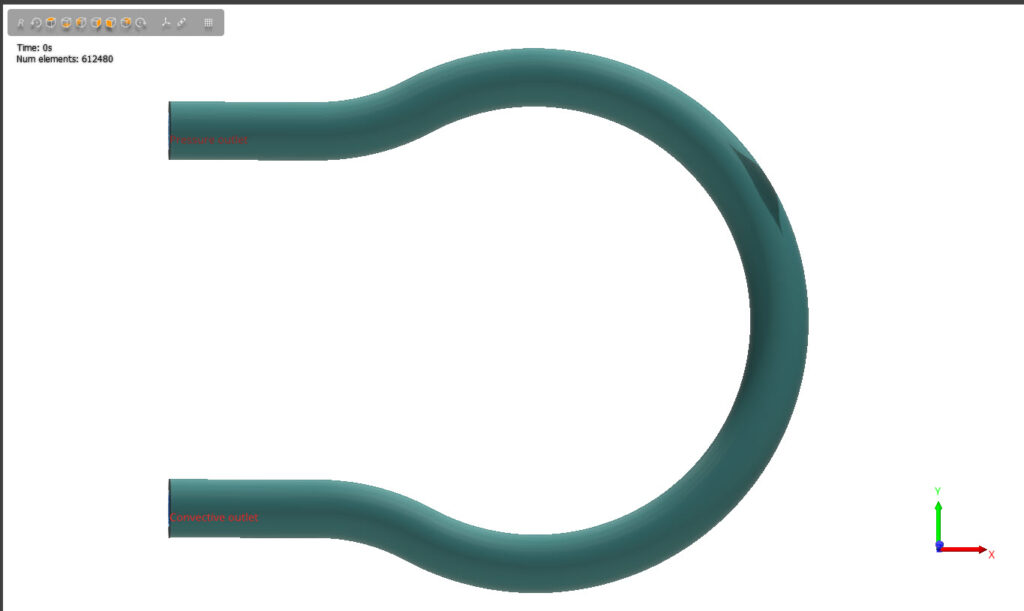
Figure 6: CFD model geometry and inlet/outlet conditions

Fluid properties

For the CFD model, water was used as the fluid, in this particular case. The relevant properties used, are given below in Table 1.

Reference density 998.3 kg/m3

Viscosity model Newtonian

dynamic viscosity 0.001 Pa s

Table 1: Properties of water for CFD domain

---

SIMULIA offers an advanced simulation product portfolio, including Abaqus, Isight, fe-safe, Tosca, Simpoe-Mold, SIMPACK, CST Studio Suite, XFlow, PowerFLOW and more. The SIMULIA Learning Community is the place to find the latest resources for SIMULIA software and to collaborate with other users. The key that unlocks the door of innovative thinking and knowledge building, the SIMULIA Learning Community provides you with the tools you need to expand your knowledge, whenever and wherever.