
Want to learn how to simulate X-ray tubes in SIMULIA Opera? Don’t miss the on-demand webinar!
Part 1 of this article briefly reviewed the operation of X-ray tubes; here in Part 2, we will examine how Opera addresses the task of simulating the main processes involved, and how this enables their efficient design and analysis.
The processes that lead to X-ray production highlight the need to generate, accelerate, transport and focus an electron beam onto a target. These are the processes that we are principally concerned with when it comes to Opera simulations.
X-ray tubes in Opera
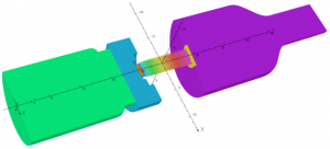
Figure 2.1 shows the components of a typical tube, as we might represent them in Opera.
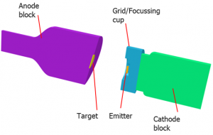
We can identify a number of typical components for inclusion in Opera models of X-ray tubes. We have a:
Source of electrons, often a hot filament thermionic emitter; latterly, cold cathode, field effect emitters have become more common. The emitters are biased at the cathode potential.
Grid – electrode close to the emitter that can be biased to switch and control the beam current. Not always present, sometimes the cathode cup is used – biased at a variable voltage below the cathode potential.
Focusing system – usually electrostatic – in many cases the focusing function is performed by shaping the cathode or cathode cup without the need for a separate, biased, electrode.
Beam target – a high atomic number material, often tungsten, rhodium or molybdenum – depending on the application. The common attributes of these materials are a high atomic number, important because X-ray yield is proportional to atomic number, and high melting point – necessary because most of the beam energy produces heat, not X-rays.
Anode – biased electrode, whose potential determines the beam energy. The anode structure provides thermal mass and a thermal conduction path away from the target. It goes without saying that the anode also provides the electrical connection to the target.
Finally, the enclosure (not shown) – providing a number of functions, including structural, voltage screening, radiation screening and filtering, and cooling. The structural enclosure might also be the vacuum vessel, or a separate glass or ceramic vacuum vessel might be contained within the enclosure.
Simulation requirements
Given the typical components of an X-ray tube, and the broad requirements of the applications, we will now consider the impact that these, and the mode of operation, place on the simulations that we need to perform.
As we have said, the X-ray tube works by accelerating and focusing electrons on to an anode, or target. So we need to be able to evaluate the fields – principally electrostatic, in this application, but magnetic fields could also be involved. Clearly, we must somehow generate the particles to be accelerated – i.e. we need emission models – and transport them to the anode, including the possibility that relativistic effects might be significant. When generating and transporting the particles in a beam, we need to be able to account for the interactions between:
- Particles and the fields – determining the trajectory of the particles in combined electric and magnetic fields, with self-consistent treatment of the effects of space-charge from the beam on the trajectories.
- Particles and surfaces – where energy will be deposited and secondary particles might be generated, along with X-rays.
- Particles and volumes – if we have residual gas, for example.
Many X-ray devices involve high beam powers, and even though the target is typically a high melting point material, such as tungsten, and the anode often rotates, thermal management can be a significant problem. Hence the thermal impact needs to be evaluated – along with the consequential stresses and deformations that occur from thermal expansion.
Opera’s field solvers are highly developed, accurate, and efficient; this is perhaps the area for which Opera is best known. The electrostatic field solver is an integral part of the Charged Particle solver, where it is combined with self-consistent space charge and trajectory simulation. The Magnetostatic field solver can provide magnetic field values that may be imported into a Charged Particle model before it is solved to enable trajectory simulation in the presence of combined fields.
The Charged Particle module includes self-consistent primary and secondary emission models, including those relevant to the types of emitters that we would expect to find in X-ray tubes. As the particles are generated and tracked, the solver accounts for the modification to the potential distribution caused by their charge – including at the surface of the emitters – modifying both the emitted current distribution and the particle trajectories. The magnetic field produced by the beam current can optionally be evaluated and included in the simulation.
Another option in a Charged Particle simulation is the inclusion of the effects of imperfect (lossy) dielectrics. If included, selected parts of the model are able to carry a bulk current, which modifies the electric potential distribution over the material, and hence modifies the electric field in the model and affects the particle trajectories.
The Charged Particle solver evaluates the beam power deposited on surfaces – as the difference between the incident power and any power emitted by secondary emission from the surface. If running under the Opera Multiphysics facility, this deposited power distribution is automatically made available to the next stage of the analysis – usually a static thermal simulation. For additional flexibility, the power distribution can also be exported in the form of standard-format ASCII data files (ie Opera table files), which may be used in, say, Opera transient thermal simulations, or third party applications. We will return to this a little later.
So how does Opera go about performing a Charged Particle simulation? If we limit the problem to static fields and ‘continuous’ beams, i.e. to timescales longer than the device time constants, then we can think of the beam as consisting of a discrete set of current tracks. The simulation task then comes down to finding the self-consistent trajectories of these current tracks. For these trajectories, the forces – caused by the interaction between the charge distribution of the beam and the electrostatic potential, and by the effective motion of the charge in the presence of a magnetic field – are balanced.
Don’t miss the on-demand webinar to learn how to simulate X-ray tubes in Opera!
We solve for the self-consistent trajectories using an iterative solution method. In the first iteration, we calculate the electrostatic field distribution due to the potential defined on the electrodes. Using this, and any applied magnetic field, we generate and track initial particles through the device. At the end of the iteration, we calculate the space-charge from the calculated beam current and velocity distribution, and assign this to the FE mesh. In subsequent iterations, the electrostatic field is re-calculated including the effects of the new space charge distribution. Particles are re-launched and trajectories are updated. This continues until convergence to the user-defined level is achieved, or the user-defined maximum number of iterations is reached.
Perhaps surprisingly, the technique is fast as well as accurate. It allows multiple species and multiple interactions to be evaluated in practicable time scales. Such is the speed and efficiency of the technique that we can often contemplate multi-variable, multi-objective optimization, where other techniques might struggle to give a single-case solution.
Emission models
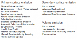
Let us return to a fundamental aspect of simulations of devices such as X-ray tubes, namely the ability to be able to generate electrons, or other particles, from emitting structures. These, of course, form the beam to be accelerated and focussed onto the anode (or target). In Opera, the physics of emission is contained in a set of models, which we call ‘emitters’. Opera includes a wide range of these emission models, the selection of which depends on the material of the emitter, its temperature and the local electric field. For example, very often in traditional X-ray tubes, the electron emitter will be a heated tungsten filament, and Opera provides a set of thermionic emitters for these cases. We sometimes also need to include the production of secondary particles that are generated when other energetic particles are incident on a surface or interact with a gas. Again, Opera includes models for these phenomena, including backscatter and true secondary generation.
Opera emitters feature flexibility and incorporate a number of attributes that allow models to be created to embody sophisticated physics. These include arbitrary particle charge and mass, and functional physical parameters. Each Opera emitter accounts for either the generation of one species of primary particle, or for the generation of a particular secondary particle from a particular incident particle. However, multiple emitters may be co-located on the same physical face, or faces, or in the same volume of a model, allowing arbitrarily complex multi-species interactions to be simulated.
The set of in-built emission models is indicated in table 2.1.
Magnetic fields
We principally expect to see electrostatic fields in X-ray tubes. However, for those instances where magnetic fields are also present, we can incorporate these in the Opera simulation. The magnetic fields may arise from a number of sources and may be included in the simulation in a number of ways.
Results extraction
If we look at what sort of result parameters that are important to designers of particle beam devices, we might arrive at a list such as that shown in table 2.2. This is perhaps not exhaustive, and some are outputs are less relevant to X-ray tube design than others, but generally, these determine the requirements for the tools that we need in the Post-Processor. Some metrics are evaluated using standard tools available in the Opera Post-Processor, but where new requirements arise, we can use the scripting capabilities of Opera to provide the needed functionality.
• Metrics of the beam – Total beam current – Beam current density and power distribution – Beam trajectories – Beam brightness and emittance – Beam moments – Phase space • Power deposition – From primary and secondary particles – Consequential thermal and stress effects • Surface erosion and material deposition – From primary and secondary particles – Consequential effects on dimensions and surface properties
Table 2.2 Typical results required from charged particle simulations
As mentioned previously, one very significant output parameter that we might want is the deposited beam power. This is evaluated in an Opera Charged Particle simulation and is available for export, and for subsequent use in, say, the Opera Thermal solver. Note that, although the Charged Particle solver is a static solver, it is possible to simulate the thermal effect of a time-varying beam – for example, a single pulse, or pulse-train – simply by applying a time function to the power loading from the Charged Particle simulation. But let’s first have a look at how we would use Opera’s Multiphysics environment to run a simple continuous beam example.
Multiphysics simulations
When setting up a multiphysics simulation, we chain the required analysis stages – simply by dragging the required solvers from the Solvers pane into the main canvas, as indicated in figure 2.2.
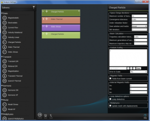
We apply the model set-up data – such as material properties, boundary conditions, etc – to a single model. All data that needs to be used in a particular stage of analysis is obtained automatically from the results of the preceding stage. All results are available in a single database, once solved.
So, for the analyses in which we are interested at the moment, we pass the beam power loading from the Charged Particle simulation to Thermal; the resulting temperature distribution is passed to the Stress analysis to determine the thermal expansion effects. Finally, a second Charged Particle analysis is run using the deformed structure from the Stress analysis. We can see some results from a simple model in figure 2.3.
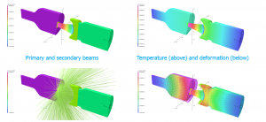
This shows the Charged Particle solution in the left-hand two images, and the resulting thermal and stress results in the two images on the right.
As mentioned earlier, we can also run a transient thermal analysis using the results of a Charged Particle simulation. Let’s take the example of a pulsed X-ray tube. Our main criterion is that the pulse is long enough – by this, we mean that the beam reaches steady state in a time much shorter than the pulse duration. We will use a similar example to that used before, as shown in figure 2.4.
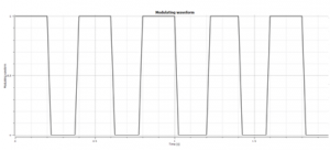
The Charged Particle simulation provides the beam power loading, which we import into an unsolved Transient Thermal database, factored by the required modulation function. In this case we used a pulse train with a repetition frequency of 2.5Hz and a 1:1 mark-space ratio.
The Transient Thermal simulation was run for a total of 2 simulation seconds, and we extracted the maximum temperature in the model every 2.5ms (note that the simulation time-step is finer than this, at 0.5ms). The input pulse train and resulting temperature are shown in figure 2.5.
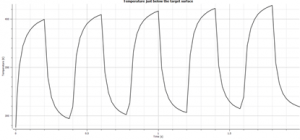
As can be seen, the maximum temperature changes rapidly as the pulse switches on and off. It is clear that the peak temperature is still rising, indicating that more simulation time-steps are required to reach steady-state.
Summary
In this article, we have briefly reviewed the operation of X-ray tubes and outlined the capabilities needed by software tools intended to facilitate their design. We have described the capabilities and features of Opera and its Charged Particle solver that make them well suited to the design task.
Among these features are:
- Accuracy and speed
- Self-consistent, particle simulation, including space charge
- A comprehensive set of particle emission models
- A comprehensive set of interactions
- Particle – field
- Particle – surface
- Particle – volume
- Powerful and flexible post-processing
We have noted that the X-ray tube design process can take advantage of Opera’s multiphysics environment, allowing Charged Particle, Thermal, and Stress analyses to be run on a single, consistent model of the device.

SIMULIA offers an advanced simulation product portfolio, including Abaqus, Isight, fe-safe, Tosca, Simpoe-Mold, SIMPACK, CST Studio Suite, XFlow, PowerFLOW, and more. The SIMULIA Community is the place to find the latest resources for SIMULIA software and to collaborate with other users. The key that unlocks the door of innovative thinking and knowledge building, the SIMULIA Community provides you with the tools you need to expand your knowledge, whenever and wherever.

Mike Hook is a SIMULIA Electromagnetics Industry Process Consultant.