Turkey Time (or Transient Thermal Analysis Tutorial) with Fidelis

It’s turkey time with our friend and guest blogger Rob Hurlston from Fidelis! In honor of Thanksgiving, he’s sharing a transient thermal analysis tutorial for cooking a turkey. Hope everyone has an enjoyable and safe Turkey Day! 

Stay tuned for more fun tutorials from Rob and Fidelis!

It’s Thanksgiving week and we’re all eagerly anticipating that perfectly roasted bird on Thursday afternoon. But how do we know whether our turkey is thoroughly defrosted and, perhaps more importantly, cooked to perfection. At Fidelis, we’re always looking for a reason to simulate – anything – and what could be more appropriate than this age-old conundrum. So if you’re looking to avoid a National Lampoon’s style disaster like this one, keep reading.

In order to get an idea of timing, we did some research and came up with some ideas for defrost time in the refrigerator and cooking time in the oven. For a turkey of target weight 15-17lbs, it turns out we need to defrost for 3-4 days and cook for between 3 and 5 hours. Because this is a transient process (i.e. time is involved) we took advantage of the transient thermal analysis capability in Abaqus. Similar to explicit for mechanical applications, this allows us to take account of time and temperature in our analysis.

The full workflow tutorial to replicate this analysis within the Abaqus CAE graphical user interface (GUI) is included in this video, but we’ll summarize the important parts here in the order that they were executed:

Model Attributes

Prior to starting this model build, it is important that we set a couple of parameters for the model as a whole. Firstly, we need to define the temperature at absolute zero, and, since we will be working in degrees Celsius, that is -273C. The Stefan Boltzmann constant also needs to be defined as 5.6×10-11 mW⋅mm-2⋅C-4.

Parts and Assembly

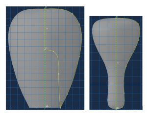
To get started, we’ll need to create some parts. Initially we freehand sketch and revolve the body of the turkey, aiming for dimensions of around 100mm in radius and 300mm in length – and don’t forget to include a cavity for the stuffing. Then the legs are made in much the same way, with dimensions around 60mm for the radius of the meat and length 200mm. It is obviously up to you to define the size of your bird, but for reference, our turkey ended up right around the 15lb mark.

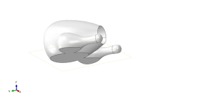
The legs are then to be assembled and combined with the turkey body using the ‘Merge/Cut Instances’ process within the Assembly module and the new part is given a flat bottom using the Create Cut: Extrude operation. Finally, we define a shell for the 350x400mm steel cooking sheet and the parts are arranged (translate ; rotate) such that the turkey sits atop of it.

Property

Fortunately, there has been a lot more research into the thermal properties of turkey than you’d ever imagine. Thank you refrigeration industry!

We managed to obtain density, conductivity and specific heat for the turkey meat and also need to define the equivalent for the steel sheet.

Turkey Density: 1.05×10-9 tonne/mm3

Turkey Conductivity: 0.41mW/mm.C

Turkey Specific Heat: 2.8×109 mJ/tonne.C

Steel Density: 7.85 x10-9 tonne/mm3

Steel Conductivity: 47.7mW/mm.C

Steel Specific Heat: 4.77×108 mJ/tonne.C

In terms of Section definitions, the turkey should be prescribed a solid Section property and the steel a shell Section property of 2mm.

Step

Given that we need to defrost and then roast the turkey, two separate steps should be defined. As mentioned earlier, these need to be 4 days (345,600 seconds) and 5 hours (18,000 seconds), respectively. We’ll want to check in on the turkey periodically, so we chose to take 100 equally spaced increments in each step of the analysis. If you’re tight on disk space, you might want to check in on your turkey less often…

Interaction

A couple of interactions must be defined for the analysis to work. Firstly, we need to apply a tie constraint between the base of the turkey and the steel sheet. Then we can apply our thermal interactions in the form of Surface Film Conditions. In Step 1 we can use a film coefficient of 0.001mW/mm2.C, which represents reasonably still air like that you’d find in a refrigerator. Our sink temperature should be 4C. Step 2 represents roasting in the oven, so we’re going to assume some convection here: 0.01 mW/mm2.C. The oven will be set to 176C for the 5-hour roasting period.

Load

There isn’t much that we need to do in the Load module, but we do need to prescribe a Predefined Field of -18C for the temperature of the initial temperature of the bird straight out of the freezer.

Mesh

The turkey geometry that we’ve produced is too complex for the mesher to assign a hexahedral mesh. That’s fine, for this analysis, we’re OK with a sloppy tetrahedral mesh and so we select Free Tet in the ‘Assign Mesh Controls’ window. With a global mesh size of 10mm , the part is ready to be meshed .

The cooking sheet shell must also be meshed, and we’re going to assign a mesh size of 5mm.

One thing to make sure of is that we’re using Heat Transfer elements throughout – DC3D10 for the tetrahedral elements of the turkey and DS4 for the shells.

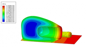
At this point, we’re ready to launch the analysis! Hopefully you can put this to good use and have some fun simulating your own Thanksgiving turkey. Of course, many aspects of this transient thermal analysis carry into all sorts of other applications too, maybe even some that are relevant to your real job?

As a provider of all of SIMULIA’s simulation products, as well as a CAE services provider that puts them to good use, we’d love to hear from you about your software and simulation needs!

Robert Hurlston, EngD, PGDip, MEng, is a Principal and Chief Engineer and co-founder of Fidelis. Throughout his career, he has worked on and led on a diverse array of projects across a range of industries. This has allowed him to sharpen his analytical proficiency, particularly in the fields of linear and nonlinear stress analysis, dynamics, fatigue, and optimization.

Rob has a strong background in materials, with a specialty in metallurgy and structural integrity engineering. His industrially based doctorate and subsequent post-docs in nuclear materials engineering saw him accumulate over a decade of real-world experience in collaboration with Serco, the University of Manchester (UK), and their partners. Rob has presented much of his work at a number of prestigious international conferences and has also published several journal papers.

Rob holds a first-class master’s degree in materials science and engineering and a postgraduate diploma in enterprise management, along with his doctorate, all of which were completed at the University of Manchester.

He is a big soccer fan and an avid golfer. He also enjoys skiing, hiking, and playing the guitar, as well as spending time with his family.