
Introduction
Multiphysics technology has been a part of the Abaqus Unified FEA product suite from the beginning. Starting with Abaqus V2 (in 1979), Abaqus/Aqua simulates hydrodynamic wave loading on flexible structures for offshore pipelines. Multiphysics simulation capabilities have been in continuous development since then are fully integrated as core functionality in SIMULIA products. The advantage of utilizing organic multiphysics capabilities, such as available in Abaqus, include the ease with which Multiphysics the Abaqus structural FEA user can solve complex problems involving multiple physics domains. For starters, the same model, same element library, same material data, and same load history are utilized for all the physics. Secondly, the Structural FEA model can easily be extended to include additional physics interaction, without the need for additional tools, interfaces, or simulation methodology.
Don’t miss the Tech Talk on August 25th. Register now!
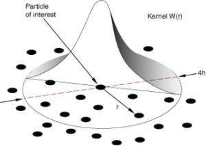
Herein, we will discuss the usage of one such capability to solve a simplified, yet realistic engineering problem: Smooth Particle Hydrodynamics (SPH), which is available on the 3DEXPERIENCE Platform as well as Abaqus Unified FEA. SPH is a versatile and powerful “mesh-free” Lagrangian computational method that was introduced in the mid-1970’s as to solve structural problems related to astrophysics and has been broadly employed in many global industries, including Defense, Marine, and Life Sciences. SPH is a continuum modeling method (like FEM) derived in the context of interpolation theory, whereby the properties at a particle (a material point, similar to an integration point in traditional finite elements) are “smoothed” over a finite region. A “kernel function” W, which as shown in Figure 1 is a function of the distance from the material point of interest, is used to approximate and smooth the Direct delta function. Additional background on the SIMULIA implementation of SPH, first released in Abaqus 6.11 and in 3DEXPERIENCE R2016x, is available from the SIMULIA/Abaqus Analysis Techniques manual.
Other Particle-based Techniques for Fluid Flow
It is important to recognize that SPH differs substantially from lattice Boltzmann method (LBM) solver approaches utilized in computational fluid dynamics (CFD) tools such as PowerFLOW or XFlow, both also available from SIMULIA. While both are particle-based methodologies and may be used to describe the physics of fluids in motion, they derive from very different approaches and treat the underlying continuum very differently. LBM is a somewhat newer simulation approach, developed in the late-1980’s from Kinetic Gas Theory. While SPH solves the standard continuum equations of motion (similar to FEA), LBM solves Boltzmann equation in a discrete velocity space. LBM therefore generally allows for a far more detailed continuum description of the fluid than is available in structural-based solvers such as Abaqus/Explicit, where the mechanical description of the fluid is limited principally to hydrodynamic equations-of-state (EOS), bulk properties (such as bulk modulus), and density.
Flow of a Water “Plug” Through a Thin “Atomizer” Pipe
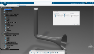
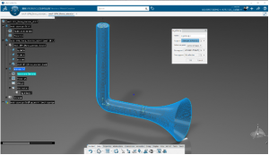
We will demonstrate the fluids modeling capabilities by outlining the process for setting-up a dynamic fluid-structure interaction simulation on the 3DEXPERIENCE Platform. (Usage of SPH in Abaqus Unified FEA is covered extensively in the Modeling Extreme Deformation and Fluid Flow with Abaqus training class.) Here, we have employed the latest release of the 3DEXPERINCE Public Cloud and utilized the Structural Analysis Engineer role. We start with a basic assembly of two products: a simple pipe with a bend and an “atomizer” fan at the end and a small “plug” or drop of fluid, as shown in Figure 2. The pipe diameter is 15-mm at the inlet and 50-mm at the exit. The entire pipe length, including the elbow, is a little over 250-mm and the inside of the pipe is assumed to be smooth. The initial water drop is 250-mm long.
We’re in the early design stage of this small component, and what we’re principally interested in is the loads on the mounting-point of the pipe under the effect of the water flowing through it. As such, rather than run a complex, fully coupled fluid-structure interaction analysis using multiple analysis codes, we can utilize the organic multiphysics simulation capabilities of the structural apps to get a good first estimate of these loads. Later, if required, we can utilize CFD tools to offer a somewhat more precise representation of the fluid.
Building of the Finite Element Representations
The Finite Element Representations (or FEMReps) for each product are used to define the FEMRep for the assembly in the Structural Model Creation app. Take notice in Figure 2 that the definitions of the individual products used in the assembly are complete, meaning that they have their own FEMReps, material definitions, section properties, and even simulation abstractions. Defining your model in this way maintains traceability of the simulation; meaning that any change to any part of the individual products will render the assembly out of date, and trigger the analyst to update and re-simulate the scenario.
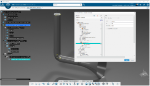
The fluid (water) is traveling in the pipe with an initial axial velocity of 35-m/s. The material behavior is defined using the linear Hugoniot form of the Mie-Grüneisen equations of state, as shown in Figure 3. This form of the model provides a hydrodynamic material model in which the material’s volumetric strength, and determines the pressure (positive in compression) as a function of the density, ρ, and the specific energy (the internal energy per unit mass), Em:p=f(ρ,Em). As we expect the fluid to begin to “atomize” or separate into droplets after it encounters the elbow, we further need to model tensile failure of the water, using the cavitation pressure of the fluid (roughly 24 MPa at room temperature). Tensile Failure has been available in Abaqus/Explicit as a keyword edit to Abaqus INP files, but as can be seen in Figure 4 is available as part of the USUP EOS definition, providing a nice enhancement to the ease of the setup process.
Defining the SPH Particle Section
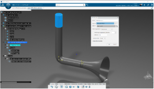
We further define the SPH particle section in the same manner, as shown in Figure 5. Note that we are able to access this definition, and all model definitions, in our assembly simply by “double-clicking” on the “SPH Particles.1” item in the specification tree at the left. The current context will change from the current app (for example, the CATIA Assembly Design app) to the Structural Model Creation app, allowing for editing as needed. Note that the SPH Particle section is defined initially based on a standard (solid element) finite element mesh (named “Sweep 3D Mesh.1”) that is converted to SPH particles at the start of the dynamic explicit analysis.

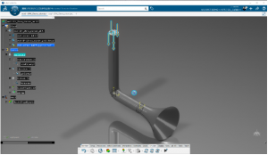
The principal abstraction in our assembly is the assumption that the pipe is a non-deformable body that is clamped at the mass-center of the pipe. This abstraction is defined in the Structural Model Creation app as shown in Figure 6.
Define the Simulation Scenario
With our individual products thus fully defined, we are now in a position to define the scenario of our simulation by using the Mechanical Scenario Creation app. We create a new simulation by selecting our assembly (the top-level product in the Specification Tree), clicking on the Compass in the upper left window, and selection the Mechanical Scenario Creation app from the resulting menu. The app will automatically create the Model-Scenario-Result (or MSR) tree that ought to be quite familiar to users of Abaqus/CAE. In this app, we define the scenario-specific quantities such as the initial velocity of the fluid, and the clamped boundary condition of the mount-point of the pipe. To allow for contact between the fluid and the rigid pipe we define a single hard-frictionless general contact interaction. The Model and Scenario are now fully-defined and ready for simulation.
Analysis and Results
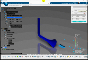
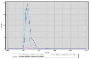
The analysis completes in about 2-hours on 4-cores of a high-end laptop computer, giving the results shown in Figure 8. Note that we’ve cut-away half of the model to show the fluid flow through the pipe. Though it seems the fluid particles are occasionally penetrating the pipe this is only an artifact of the rendering, as the definition of the particles is based on the centroid. The loads in the three axial directions at the clamped point of the pipe are given in Figure 9. We see that the loads on this clamp peak at approximately 200-N, meaning that we ought to design our restraint system to handle at least that level of load.
For further discussion of this workflow, together with an overview of the fluids analysis in Abaqus/Explicit using the Coupled Eulerian-Lagrangian modeling technique, don’t miss the August 25th Tech Talk on this topic: Fluids Modeling in Abaqus: CEL and SPH in Abaqus/Explicit.
SIMULIA offers an advanced simulation product portfolio, including Abaqus, Isight, fe-safe, Tosca, Simpoe-Mold, SIMPACK, CST Studio Suite, XFlow, PowerFLOW and more. The SIMULIA Community is the place to find the latest resources for SIMULIA software and to collaborate with other users. The key that unlocks the door of innovative thinking and knowledge building, the SIMULIA Community provides you with the tools you need to expand your knowledge, whenever and wherever.

Jon is a SIMULIA IPS Structures Industry Process Expert.