
The Santa season is upon us and we’re helping spread some holiday cheer with our friend and guest blogger Rob Hurlston from Fidelis! In honor of Christmas, he’s using membrane elements and explicit analysis to find out how fast Santa’s sack travels down the chimney, and most importantly, how all the gifts stay intact! We hope everyone has an enjoyable and safe holiday season!
Stay tuned for more fun tutorials from Rob and Fidelis in 2021!
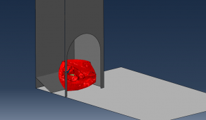
Christmas is fast approaching, and we all know what that means! Santa is on his way! Of course, the big man’s preferred choice of delivering gifts is down the chimney, but has anyone ever wondered what happens when that famous red sack hits the fireplace? We decided to find out by simulating the fall using Abaqus/Explicit and taking advantage of membrane elements to get the floppy, fabric behavior of that sack just right! If you’ve ever wondered why we do all this work drop testing electronics before they go to market, now you know.

We made some estimates of the size of the bag and added a few boxes and (maybe) a tennis racket for one lucky boy or girl on Christmas morning, but will the survive the fall? 8 meters is the typical height of a chimney on a 2-story house, and we expect a free fall to result in an eventual velocity of around 12.5m/s… that can’t be good for the gifts, right? The membrane elements we use to simulate the sack maintain load carrying capability in their plane, but no bending, which we consider the main learning outcome of this tutorial.
The full workflow tutorial to replicate this analysis within the Abaqus/CAE graphical user interface (GUI) is included in this video, but we’ll summarize the important parts here in the order that they were executed:
Parts and Assembly
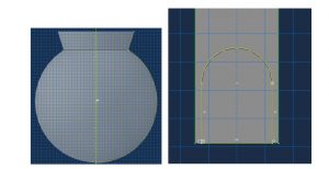
As always, we’ll need to create some parts within the Abaqus/CAE GUI. We start with the sack, which should be a revolved (almost) sphere with a collar that measures around 800mm in diameter… remember, this sack has to fit a lot of gifts in it! Don’t worry about the shape, once we preload the sack with gifts, it’ll start to look a lot less like a cauldron. The floor is a 4,000mm square rigid shell and the chimney itself is a 1,000×1,200mm extruded rigid shell. Don’t forget to cut the opening using the Create Cut: Extrude operation.
Gifts can be created as solid parts and can really be any shape you choose, as long as they fit in the sack you just made!
To assemble the parts, use the Translate and Rotate Instance operations within the Assembly module. You can leave the gifts floating in space for now, the preload step will take care of them for you.

Property
The properties of the sack itself came from some tested fabric and should be applied using a shell membrane section of 1mm thickness. The gifts use 3D homogenous material properties and these are close to cardboard.
Sack Density: 1×10⁻¹⁰ tonne/mm3
Sack Elastic: Young’s Modulus = 25MPa, Poisson’s Ratio = 0.3
Gift Density: 5×10⁻¹⁰ tonne/mm3
Gift Elastic: Young’s Modulus = 300MPa, Poisson’s Ratio = 0.3
Gift Plastic:
Yield Stress (MPa) Plastic Strain
2 0
3 0.08
Step
We will actually be using two steps for this analysis. The first one is required in order to preload the sack and have it take it’s shape. This will be run for 0.5 seconds and have a target time increment of 1×10⁻⁶s.
Then it’s time to drop the sack. We know from some hand calculations that it will take just over 1 second for the sack to fall the 8m from stationary, so running the analysis for 2 seconds will provide plenty of time for smashing and rolling. We also like to output field data 120 times per step in evenly spaced increments, just so the resolution of the video is acceptable.
Interaction
A couple of interactions must be defined for the analysis to work. Firstly, we need to apply a Rigid Body Constraint between the discrete rigid parts and a predefined control node or Reference Point. Then we can apply General Contact to the entire assembly – and don’t worry about contact parameters, the Abaqus defaults are fine for this analysis.
Load
For the sack and gifts to fall, we must prescribe Earth’s gravity to the analysis. That means a Load of type Gravity and value -9,800 mm/s2 in the negative-z direction.
And it’s not just ‘loading’ that is defined within the Load module of CAE. Boundary Conditions also need to be specified here, and in this case, we need an Encastre condition on the Reference Point of the discrete rigid surfaces that we made earlier. That will ensure that our floor and chimney stay exactly where they are throughout the entire analysis. We also need to constrain the top of the sack during the preload step, and we do that with an Encastre boundary condition also – don’t forget to turn this off in the BC Manager in the Drop step to ensure we see the sack fall!
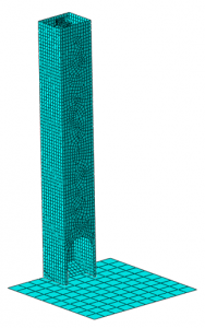
Mesh
Most of the parts can simply be meshed using Abaqus default settings. However, we do need to ensure that we use membrane elements for the sack, and that can be done using the Assign Element Type operation and selecting ‘Membrane’. We also want to use the Assign Mesh Controls feature to seed the sack with mesh of ~20mm. This helps ensure that the sack is able to deform in a realistic way.
Run The Analysis
At this point, we’re ready to launch the analysis! Hopefully you’ll find this entertaining and a somewhat helpful learning opportunity. The simulation doesn’t take too much time at all to run, so why not play with some of the parameters and initial position of the gifts. You’ll be surprised at the differences you see based on inertia. Hey, it might even be relevant to your real job?
As a provider of all of SIMULIA’s simulation products, as well as a CAE services provider that puts them to good use, we’d love to hear from you about your software and simulation needs!
Robert Hurlston, EngD, PGDip, MEng, is a Principal and Chief Engineer and co-founder of Fidelis. Throughout his career, he has worked on and led on a diverse array of projects across a range of industries. This has allowed him to sharpen his analytical proficiency, particularly in the fields of linear and nonlinear stress analysis, dynamics, fatigue, and optimization.
Rob has a strong background in materials, with a specialty in metallurgy and structural integrity engineering. His industrially based doctorate and subsequent post-docs in nuclear materials engineering saw him accumulate over a decade of real-world experience in collaboration with Serco, the University of Manchester (UK), and their partners. Rob has presented much of his work at a number of prestigious international conferences and has also published several journal papers.
Rob holds a first-class master’s degree in materials science and engineering and a postgraduate diploma in enterprise management, along with his doctorate, all of which were completed at the University of Manchester.
He is a big soccer fan and an avid golfer. He also enjoys skiing, hiking, and playing the guitar, as well as spending time with his family.

Katie is the Editor of the SIMULIA blog, an expert in engineering and scientific communication, and a strategic digital marketer. Katie has a BA in English and Writing from the University of Rhode Island and a MS in Technical Communication from Northeastern University. She is also a proud SIMULIA advocate, passionate about democratizing simulation for all audiences. Katie is a native Rhode Islander who lives just outside of her favorite city, Providence. She is a true New Englander and loves sharing all the cool things NE has to offer. She enjoys a variety of hobbies including history, astronomy, science/technology, science fiction, true crime, fashion and anything associated with nature and the outdoors. She is also mom to a 6-year old budding engineer and two crazy rescue pups.