This blog post was originally published in October 2020, but smashing pumpkins never gets old!
We’ve got a special Halloween treat! Guest blogger Rob Hurlston from Fidelis is sharing his ductile damage tutorial for a pumpkin smash. Hope everyone has an enjoyable and safe Halloween!
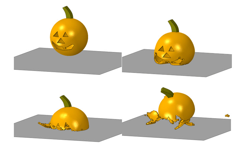
We all love Halloween. The cooler weather, the candy and, of course, the pumpkins. So, in the spirit of the season, we at Fidelis decided we’d try to recreate the never-gets-old feeling you get when you see a pumpkin smash into pieces on the ground having been dropped from a great height. And what was the first tool we thought about in order to pull this off? Abaqus of course!
We settled on a 5m drop, which is equivalent to something like a second-story window – hence something we can all recreate at home if we feel the need to carry out an impromptu correlation study. With this being a highly dynamic event, we utilized Abaqus’ explicit solver and, to ensure the pumpkin actually smashed when it hit the ground, we took advantage of the ductile damage feature. Typically, this methodology might be reserved to predict failure in metallic components of a car or airplane, but a little creative tuning of the parameters allowed us to generate reasonably true-to-life behavior of the classic pumpkin drop.
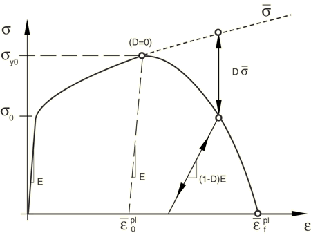
For some background, the ductile damage method allows us to prescribe a reduction in both yield strength, Dσ, and elasticity, (1-D)E, as strain increases beyond a predefined threshold (see figure). Eventually, the element reaches zero load carrying capability and is effectively removed from the analysis.
The full workflow tutorial to replicate this analysis within the Abaqus CAE graphical user interface (GUI) is included in this video, but we’ll summarize the important parts here in the order that they were executed:
Parts and Assembly
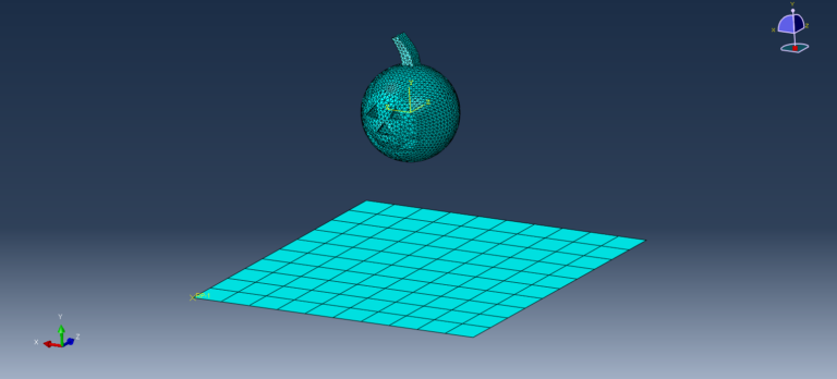
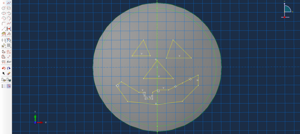
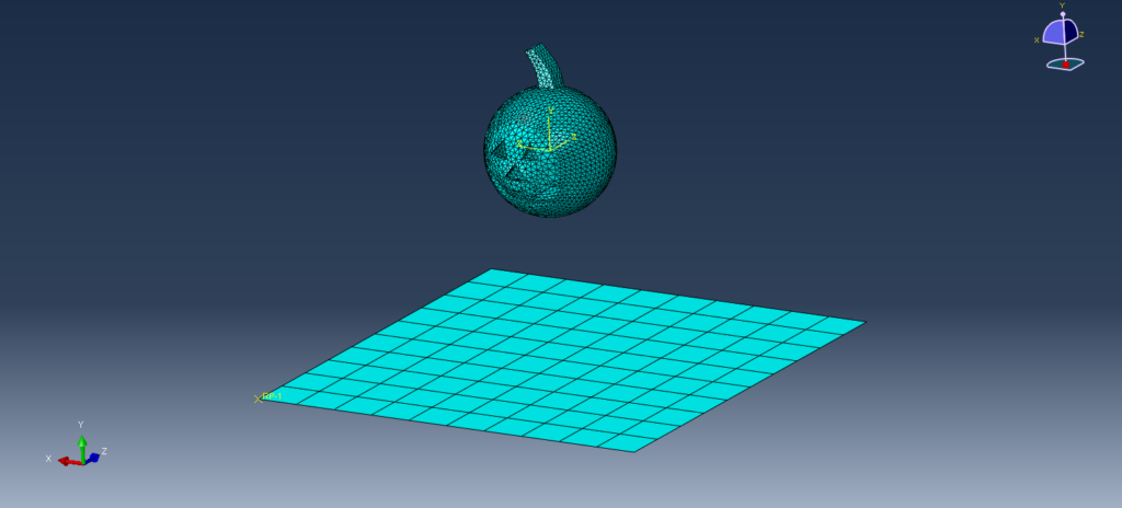
First of all, we must create the parts . A solid revolved hollow sphere of diameter 600mm and wall thickness 25mm represents the main body of the pumpkin. To ‘carve’ the face, the ‘Create Cut: Extrude’ feature should be employed – and you can go wild, freehand, with the sketching tools. I even gave my pumpkin a snaggly tooth.
A solid extrude is generated for the stem and that is combined with the pumpkin body using the ‘Merge/Cut Instances’ process within the Assembly module. Finally, a discrete rigid shell is defined for the ‘floor’ and the parts are arranged (translate; rotate) such that the pumpkin begins its journey from a round 1x it’s diameter from its landing zone.
Property
As mentioned earlier, the properties for the pumpkin were somewhat tuned, but we tried to base them in some sensical assumptions. Density, for example, was taken from measured data at 4.8 g/cm3 (or 0.48×10⁻⁹ tonnes/mm3). Other parameters can be seen below:
Elastic: Young’s Modulus = 20MPa, Poisson’s Ratio = 0.3
Plastic :
Yield Stress (MPa) Plastic Strain
2 0
3 0.1
Ductile Damage: Fracture Strain = 1×10⁻⁵, Stress Triaxiality = 0, Strain Rate = 0
Damage Evolution: Type = Displacement, Softening = Linear, Degradation = Maximum, Displacement at Failure = 5×10⁻⁵ mm
Step
The step is, of course, Dynamic Explicit in nature, so the step type should be selected accordingly. Time is set to 1 second and mass scaling defined to give an increment time target of 1×10⁻⁶ s.
Interaction
A couple of interactions must be defined for the analysis to work. Firstly, we need to apply a Rigid Body Constraint between the discrete rigid floor and a predefined control node or Reference Point. Then we can apply General Contact to the entire assembly – and don’t worry about contact parameters, the Abaqus defaults are fine for this analysis.
Load (And A Predefined Field)
When the pumpkin lands, we don’t just want it to bounce back into space, we want it to flop and fall, and so we must prescribe Earth’s gravity to the analysis. That means a Load of type Gravity and value -9,800 mm/s2 in the direction of the y-axis. Further, we don’t want to have to extend the analysis further than is necessary, so we define the velocity that the pumpkin would be travelling had it been dropped from a height of 5m in the form of a Predefined Field. In this case, that is -9,900 mm/s.
It’s not just ‘loading’ that is defined within the Load module of CAE. Boundary Conditions also need to be specified here, and in this case, all we need is an Encastre condition on the Reference Point of the discrete rigid surface that we made earlier. That will ensure that the floor stays exactly where it is throughout the entire analysis.
Mesh
The pumpkin geometry that we’ve produced is too complex for the mesher to assign a hexahedral mesh, which is – fittingly – why it shows up as orange initially. For this analysis, we’re fine with a sloppy tetrahedral mesh and so we select Free Tet in the ‘Assign Mesh Controls’ window. With a global mesh size of 25mm, the part is ready to be meshed.
The discrete rigid must also be meshed, and we let CAE do all the work here, simply clicking the ‘Mesh Part’ button and moving on.
It should be noted that the STATUS Field Output is required so that the spent elements are removed from the visualization of the analysis and we should output results at 200 evenly spaced intervals.
At this point, we’re ready to launch the analysis! Hopefully you can have a bit of fun with this ghoulish tutorial, and maybe take something away that helps you in future simulation efforts, particularly in the form of explicit analysis that includes ductile damage.
As a provider of all of SIMULIA’s simulation products, as well as a CAE services provider that puts them to good use, we’d love to hear from you about your software and simulation needs!

Robert Hurlston, EngD, PGDip, MEng, is a Principal and Chief Engineer and co-founder of Fidelis. Throughout his career, he has worked on and led on a diverse array of projects across a range of industries. This has allowed him to sharpen his analytical proficiency, particularly in the fields of linear and nonlinear stress analysis, dynamics, fatigue, and optimization.
Rob has a strong background in materials, with a specialty in metallurgy and structural integrity engineering. His industrially based doctorate and subsequent post-docs in nuclear materials engineering saw him accumulate over a decade of real-world experience in collaboration with Serco, the University of Manchester (UK), and their partners. Rob has presented much of his work at a number of prestigious international conferences and has also published several journal papers.
Rob holds a first-class master’s degree in materials science and engineering and a postgraduate diploma in enterprise management, along with his doctorate, all of which were completed at the University of Manchester.
He is a big soccer fan and an avid golfer. He also enjoys skiing, hiking, and playing the guitar, as well as spending time with his family.

Katie is the Editor of the SIMULIA blog, an expert in engineering and scientific communication, and a strategic digital marketer. Katie has a BA in English and Writing from the University of Rhode Island and a MS in Technical Communication from Northeastern University. She is also a proud SIMULIA advocate, passionate about democratizing simulation for all audiences. Katie is a native Rhode Islander who lives just outside of her favorite city, Providence. She is a true New Englander and loves sharing all the cool things NE has to offer. She enjoys a variety of hobbies including history, astronomy, science/technology, science fiction, true crime, fashion and anything associated with nature and the outdoors. She is also mom to a 6-year old budding engineer and two crazy rescue pups.