Gasket Simulation in Abaqus

What is a Gasket?

The primary uses of a gasket are to provide a robust seal between two flanges, to endure thermal and mechanical loading, to resist exposure to different materials, and, to ensure overall system integrity. Important examples include head and valve cover gaskets in combustion engines.

Why Do We Use Gaskets?

A frequently asked question is, “Why not clamp the flanges directly together instead of using a gasket?”

Despite the simplicity of this approach, it isn’t the most economical solution. Clamping flanges would entail using more bolts, smooth machining of flanges (inflating the costs), or potentially welding, which introduces complexities during disassembly.

Gaskets play a definitive role in preventing leaks and ensuring the integrity of the sealed components. Understanding their behavior and properties for complex assemblies and loading conditions is crucial for accurate engineering analysis.

What are Typical Applications of Gaskets?

Typical applications include:

• In internal combustion engines, gasket applications include head gaskets, exhaust manifold gaskets, valve cover gaskets and intake-manifold gaskets.
• Medical devices
• Food packaging
• Cell phones  
• Fuel cells

What Types of Gaskets Do We Use?

Gaskets come in different types, including metallic and non-metallic gaskets. Metallic gaskets, crafted from steel, aluminum and copper, offer durability and resilience. Non-metallic gaskets can be crafted from fibrous materials, composites, molded rubber, and graphite. Each material type is chosen based on its specific properties and the application’s requirements.

Challenges in Gasket Analysis

With their intricate geometries and complex behaviors, especially in the mechanical response along the thickness direction, gasket simulation can be challenging yet critical in advanced engineering analysis.

• The in-plane dimensions often differ significantly from the thickness, which could lead to complex meshing processes.
• Finite element analysis could require a sophisticated model to account for the complicated through thickness behavior, complex calibration & meshing, and result in an elaborate model with millions of degrees of freedom.

Additionally, gaskets must be considered in conjunction with the overall structure with ceiling analysis addressing the compliance of flanges and fasteners.

A holistic approach is essential to address these complexities, acknowledging the gasket’s role within a broader structural context.

Abaqus Solution: Gasket Elements

Abaqus introduces a dedicated solution with its gasket elements, which are specifically to model gaskets. These elements improve and simplify the meshing and modeling challenges associated with gaskets by:

• Improving the mesh quality by eliminating the need for excessively refined solid element meshes.
• Streamlining mesh creation using one layer of gasket elements through the thickness.
• Simplifying mesh modification by using the profile to determine the meshing requirements.
• Leveraging constitutive modeling to tackle complex gasket thickness behavior regarding the mechanical response through the thickness. The data can be input from test data or the results of finite element models of the gasket cross-section.

The Pretension Section in Abaqus/Standard is a convenient approach to applying bolt loading. Alternatively, Abaqus/Standard and Abaqus/Explicit offer connector element technology.

Types of Gasket Elements in Abaqus

Abaqus offers two primary formulations for gasket elements: regular gasket elements and normal-only gasket elements.

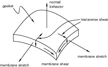
Regular gasket elements have 3 degrees of freedom per node that can model an uncoupled membrane, transverse shear, and through-the-thickness behaviors,

Normal-only gasket elements have one degree of freedom. They model through-thickness behavior only. Normal-only gasket elements are more numerically cost-effective than regular ones but aren’t as common.

Regular gasket element properties:

• All behaviors can include thermal expansion.
• Membrane and transverse shear behaviors are elastic.
• Through-thickness behavior can be plastic and have permanent creep deformation or follow a damaged elasticity response.

Both types of gasket elements can be used to model three-dimensional, axisymmetric, and planar problems. The gasket elements can be applied in static simulations, dynamic simulations, frequency simulations, or frequency extractions, and they are formulated for minor strains and small displacement calculations.

Gasket Element Formulations

Abaqus/Standard contains various element types, including elements with two, four, and eight nodes. These elements can be utilized in static, dynamic, static perturbation, quasi-static, and frequency simulations, catering to diverse engineering scenarios.

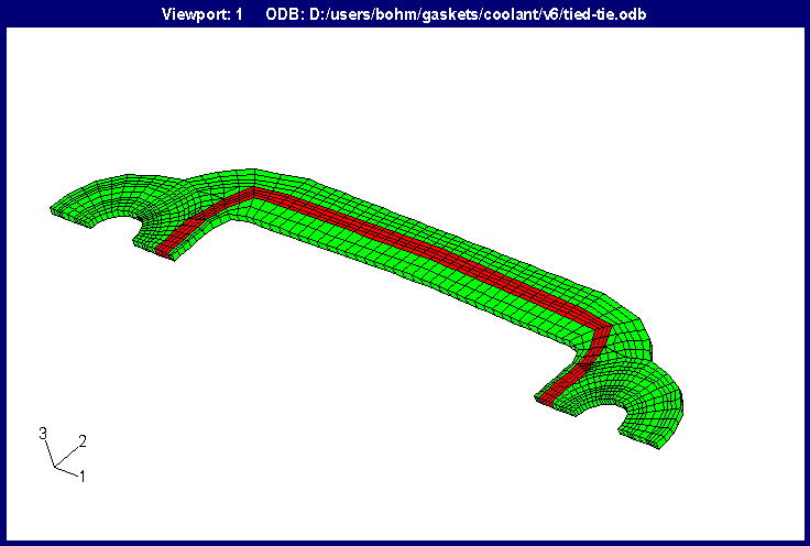
Often, gasket meshes have one gasket element through the thickness. The different colors in the gasket mesh shown here represent different gasket behaviors. The red mesh has a different gasket behavior from the green mesh.

Dynamic gaskets have damping defined by viscoelastic properties. There are gasket elements that have temperature degrees of freedom at their nodes, allowing heat transfer through the thickness direction.

Gasket elements are formulated for globally minor strains and small-displacement calculations but can be used in large-displacement calculations. Gasket elements are not ideal for use if they undergo a significant rotation because local directions do not rotate. Gasket elements can have large closures; the top can pass through the bottom if needed.

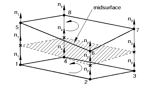
• Area elements have nodes defining the face on the top and bottom surfaces of the gasket.
• The normal goes from the bottom to the top and defines the thickness direction.
• The thickness of the gasket is calculated from the nodal locations, or it can be specified directly on the Gasket Section option.
• The default thickness of the gasket elements, the local 1-direction, is calculated by Abaqus using the nodal coordinates.
• The user can override this default local 1-direction for a group of gasket elements by using the Gasket Section option.
• The local 1-direction can be specified on a nodal basis using the Normal option.
• The direction cosines of the thickness directions obtained at the nodes of gasket elements are listed in the printed output (.dat) file.

Gasket element connectivity can differ from solid element connectivity. Numbering the nodes of the gasket is crucial since it defines the gasket’s normal direction. If necessary, use the solid element numbering parameter on the element to work around this difference. This can be convenient if the mesh generator does not support gasket elements or in thermal stress analyses where continuum elements are used to model the heat conduction in the gasket.

Fortunately, Abaqus/CAE supports gasket elements. The user can make a gasket mesh with the correct thickness direction; however, you may have to rearrange the nodal ordering on the element definition to get the correct thickness direction in some cases. Output to the data (.dat) and output from Abaqus/Viewer will use the normal gasket element connectivity.

Example

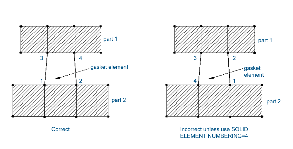
Here is an example showcasing the correct way of numbering a gasket element. The right-hand picture defines the element in the order 1-2-3-4, which only works for a plane strain element or a plane stress element, CPE4 or CPS4.

In the context of a gasket element, the thickness direction must extend from the bottom flange to the top flange. Hence, a crisscross connectivity pattern is imperative. So, if you wish to use the right-hand picture’s numbering method, you would have to declare that solid element numbering equals four. This would tell Abaqus to consider the fourth side of this element, defined as an ordinary element, as the bottom of the gasket.

It is crucial to verify the properties of the gaskets before integrating them into computational models, especially when undertaking the simulation of intricate and expansive systems.

Gasket Element Geometry

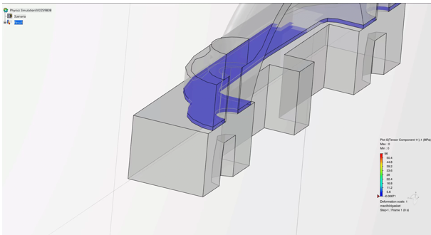
Consider the example below to model our complex gasket with a simplified mesh. The left image shows a cross-section of our complex gasket geometry in section A-A, featuring strategically placed bumps to induce ceiling pressure. However, a gap in the central region requires substantially depressing the bumps to reach the gasket body.

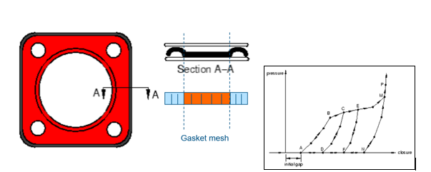
Our approach involves modeling this cross-section at the bottom to represent our gasket mesh. We exert pressure on the section to account for the gap and bumps, determining the force needed for gasket closure. This is achieved by defining a pressure closure curve within the element in Abaqus, accommodating complex mechanical responses in the thickness direction, including the gap effect. The pressure closure definitions in Abaqus allow us to account for the complex mechanical response in the thickness direction, including the effect of the gap.

Due to differences in the gasket’s middle cross-section and bumps, we define distinct behaviors for each scenario. Gasket definitions in Abaqus/CAE are achievable, with some details obscured for simplicity. Abaqus/CAE offers a comprehensive toolset for gasket definition.

Furthermore, the 3DEXPERIENCE platform supports gasket behavior in the material definition app. This integration enhances the versatility of gasket modeling within the broader computational framework.

Gasket Thickness Behavior

Gasket behavior in Abaqus is defined using pressure closure curves, material definitions, and the choice between damage and elastic-plastic behaviors. The pressure closure curve is obtained by testing the gasket in a machine and extracting the necessary data to define the behavior.

Abaqus provides options for inputting how the gasket area changes, particularly for line gaskets. This data is then used to define the gasket behavior, with two basic types: damage and elastic-plastic. The damage type involves a nonlinear elastic response that may include the effect of damage, while the elastic-plastic type includes a plastic or residual closure upon unloading.

What is Damage Behavior?

TYPE=DAMAGE defines a non-linear elastic response that may include the effect of damage. INTERPOLATION=DIRECT is used if there is a problem with unloading curves not following the input unloading curves.

If, for instance, a gasket exhibits unexpected behavior, deviating from the specified curves, it is advisable to explore this new option.

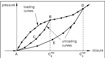
The resulting thickness behavior closely resembles the damaged elastic response observed in hyperelasticity, known as the Mullins effect. Upon loading the gasket to point B and subsequently unloading, if damage unloading is defined, the response returns elastically to point A. The damaged curve is traversed upon reloading, and the process continues accordingly.

A primary loading curve is defined for this type of thickness response, accompanied by a set of unloading curves. Abaqus employs interpolation to derive the corresponding unloading behavior when unloading occurs from an intermediate pressure.

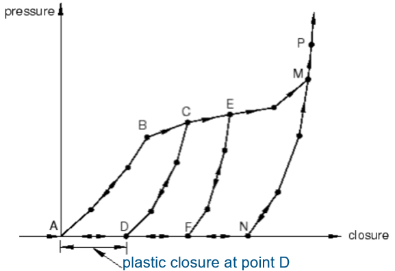
What is Elastic-Plastic Behavior?

Elastic-plastic behavior in Abaqus exhibits a plastic or residual closure upon unloading, akin to elastic-plastic materials. The software offers options to define yield points and modify interpolation for precise gasket behavior in simulations.

The default plasticity onset follows the 10% rule, allowing users to customize this criterion based on preferences. Opting for “type equals damage” is often less troublesome, especially if the gasket is not fully unloaded.

Abaqus supports various material options, including user-defined materials, for gasket elements, with the ability to specify dynamic stiffness and damping directly in the thickness behavior. The creep option is available for creep analysis as a sub option of gasket behavior or material options.

Gasket Element Output Variables

When analyzing output for a gasket element, the critical parameters include the ceiling pressure, denoted as S11. This designation applies, for example, to an element like GK3D8CS. For line gasket elements ceiling pressure is represented by E11.

E11 signifies the gasket closure, measured in units of length specific to the gasket element. While additional variables can be extracted from the gasket, the most commonly examined are S11 and E11, capturing the pressure closure.

For users seeking more customized output variables, creating user-defined output variables is possible using user output variables and the subroutine UVARM. It’s worth noting that recent Abaqus releases support gfortran for LINUX users.

Practical Tips for Gasket Element Usage

Practical tips for effective gasket element usage involve verifying gasket behavior and convergence characteristics.

Set up a single gasket element model to scrutinize its behavior by pushing it down, unloading it, and confirming the pressure closure behavior. This precaution prevents the discovery of discrepancies in gasket behavior after running a large and intricate model.

This approach is beneficial for any novel features introduced into an Abaqus simulation. It’s crucial to verify the performance of complex material models, connector element behaviors, etc., with simplified models before incorporating them into more extensive simulations.

For gaskets, a comprehensive test involving the entire gasket allows for the verification of correct gap behavior and ensures sealing pressure only occurs once the gaps are appropriately closed.

Technical issues can arise with gasket elements, particularly in cases where elements are unsupported. An unsupported gasket element refers to a situation where a portion of the gasket extends across a gap, such as a hole in a flange, without proper support. This condition can lead to problems during analysis.

To address this, there is an option called stabilization stiffness in the gasket section specifically designed to manage unsupported gasket elements. You can identify unsupported gasket element nodes during a data check by examining the printed output file for the “no intersection” text.

A small amount of stiffness is applied to mitigate numerical ill-conditioned problems arising from an initial gap. Abaqus defaults to using the slope beyond the gap multiplied by 0.001 to determine the gap stiffness.

However, this may result in excessive stiffness and noticeable ceiling pressure on the gasket body. To address this, the tensile stiffness factor option, part of the gasket thickness behavior, allows users to control and potentially reduce this factor, ensuring more accurate results.

Conclusion

Gasket simulation in Abaqus/Standard presents numerous challenges due to the intricate geometry and complex behavior of gaskets. Using gasket elements in finite element analysis is crucial for accurately capturing the behavior of gaskets under various loading conditions.

Abaqus offers a powerful solution for gasket analysis, overcoming traditional challenges associated with finite element modeling. Engineers can achieve more efficient and accurate simulations by incorporating specialized gasket elements and thickness behavior definitions, improving product designs and reliability.

To learn more about mastering gasket simulations with Abaqus/Standard, we invite you to access our recorded session here.

---

Interested in the latest in simulation? Looking for advice and best practices? Want to discuss simulation with fellow users and Dassault Systèmes experts? The SIMULIA Community is the place to find the latest resources for SIMULIA software and to collaborate with other users. The key that unlocks the door of innovative thinking and knowledge building, the SIMULIA Community provides you with the tools you need to expand your knowledge, whenever and wherever.