
The SIMULIA Blog is committed to providing high-quality simulation content that is technical and digestible for a broad audience of simulation enthusiasts. And that means connecting SIMULIA experts to our users by giving them a platform to educate and inform. Our newest series will focus on very technical concepts and simulations, delving deep into a particular topic. The following article, about various approaches for Reduced Order Model (ROM) creation in electrical machines, was written by Christian Kremers, Adrian Scott, and Nikolas Weber and was first published in automotive CAECompanion 2021/2022.
The Finite Element Method (FEM) is a versatile, accurate and widely accepted method to simulate and analyze different aspects of the electromagnetic performance of electrical machines. However, there are also many aspects for which it is more efficient or rather the only possible approach to solve them in a system simulator, where electric circuits and mechanical subsystems can be simulated as one coupled system. This requires a representation of the electrical machine, which behaves in all regards as the FEM model but with a considerable reduction in computational complexity.
The generic term for such a model is reduced order model or short ROM. In the following, several approaches to construct ROMs by means of FEA will be investigated and compared with each other in terms of accuracy, performance, convergence and energy conservation properties. The machine used for this comparison is a 3-phase interior permanent magnet synchronous machine (IPMSM) with a rated peak current Irated = 195 A, a rated torque Trated = 340 Nm and 4 pole pairs. All FEM results have been obtained in 2D using CST Studio Suite® [1] under the assumption of loss less operation. The system simulator used for the comparison was Dymola [2], a system simulator based on the Modelica language.
Approaches to obtain ROMs
All ROMs have in common that they map the input quantities, namely the currents and the rotor angle, onto the output quantities, magnetic flux linkages and torque. However, the mapping can be based either on phase quantities or alternatively on their respective quantities in the DQ-coordinate frame. The transformation between the two coordinate frames is given by the so called dq0-transformation [3]. No matter what coordinate frame is chosen, first a discretization of the input space (currents and rotor angle) is required to then capture the outputs (flux linkage and torque) as result of FEM analysis. After having simulated the discrete mapping between inputs and outputs, as next step a continuous mapping must be created for use in the system simulator.
In particular both a creation of lookup tables in phase- as well as in DQ-coordinate frame has been performed. To make the mapping continuous, a requirement for system simulation, the lookup tables, being phase- or DQ-ones, have been interpolated both linearly as well as with an Akima spline.
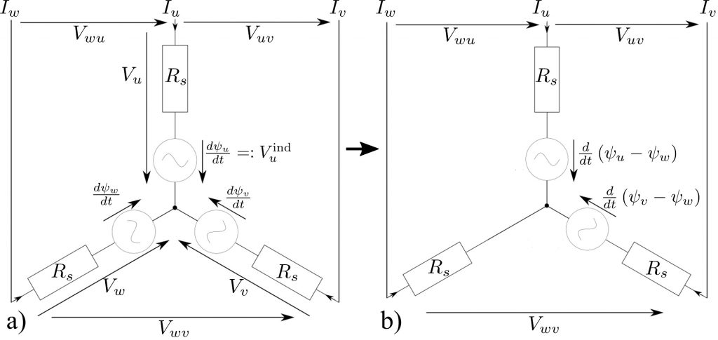
The grid for creating the lookup in terms of phase quantities was generated in the following way: The phase currents Iu and Iv have both been swept in 21 steps from -1.2 ⋅ Irated to 1.2 ⋅ Irated. Assuming a star connection of the 3 phases (see Fig. 1a) the 3rd phase current is given by Iw = -(Iu + Iv). For each of the resulting 21 ⋅ 21 = 421 current vectors (Iu, Iv, -(Iu + Iv )) the rotor has been rotated in 0.75° steps from 0° to 90° such that 120 positon steps per electrical period have been performed. The FEM outputs for each grid point are (ψu, ψv, ψw, T) where ψi stands for the flux linkage in the i-phase and T for the torque. When creating an interpolated lookup table from this data it is advantageous to reduce the degree of freedom by the transition of the circuit representation shown in Fig. 1a to the one in Fig. 1b. This transition does not change both line voltages Vij and phase currents Ii. Therefore the outer behavior of the machine is not altered at all but one should keep in mind that there is no longer any way to obtain the phase voltages.
The grid in DQ-coordinate frame is generated with the same 120 position steps as above but with 21 current steps both in Id and Iq from -1.2 ⋅ Irated to 1.2 ⋅ Irated. The FEA analysis is driven with the phase currents obtained by transforming (Id, Iq) into phase currents by the dq0 transformation. The output of the FEA is as above (ψu, ψv, ψw, T) but instead of using this data as is, the same dq0-transformation which transforms the currents is used to transform the flux linkages as well. However, the 0-component of the flux linkage does not vanish since it is not perfect balanced anymore. But using the transition from Fig. 1, one can remove the impact of the 0-component and therefore the output data for the lookup is made of (ψd, ψq, T).
To interpolate the lookup tables we have used NDTable from the SDF library shipped with Dymola. Linear and Akima spline interpolation used here are directly available in NDTable.
One additional approach for creating a machine’s ROM is the one shipped with CST Studio Suite®. The grid calculated by FEM analysis is exactly the same as in the DQ-case described above. However, the idea is not to interpolate fluxes and torque independently but instead interpolating a vector-valued function f(Id, Iq, θ) = (ψd, ψq,T) in such a way that energy-conservation is satisfied by construction. CST Studio Suite® encapsulates this type of ROM into a functional mockup unit (FMU) [4], which can be directly imported into Dymola.
Results
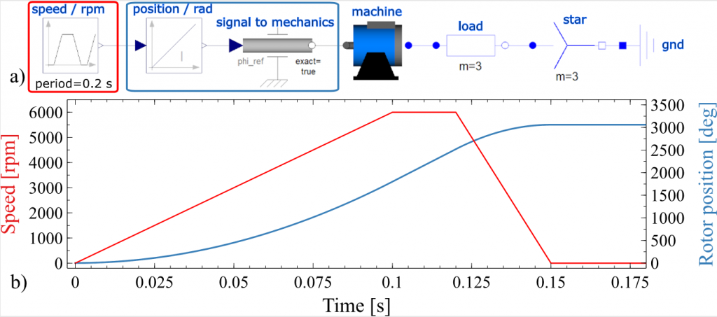
The schematic of the common test case for the different implementations of ROMs is shown in Fig. 2a. A speed profile (Fig. 2b) is applied on the shaft of the machine and a load resistance of per phase is attached. Now the underlying ROM of the machine itself is replaced with ROMs of the different flavours described above.
The resulting torques and interlinked flux linkages ψu – ψw ≔ ψuw are shown in Fig. 3. The reason to look at ψuw as a relevant quantity is justified by Fig. 1b which shows the electric part of the machines schematic implemented in all of the different ROM approaches as well as the FEM reference (solid red).
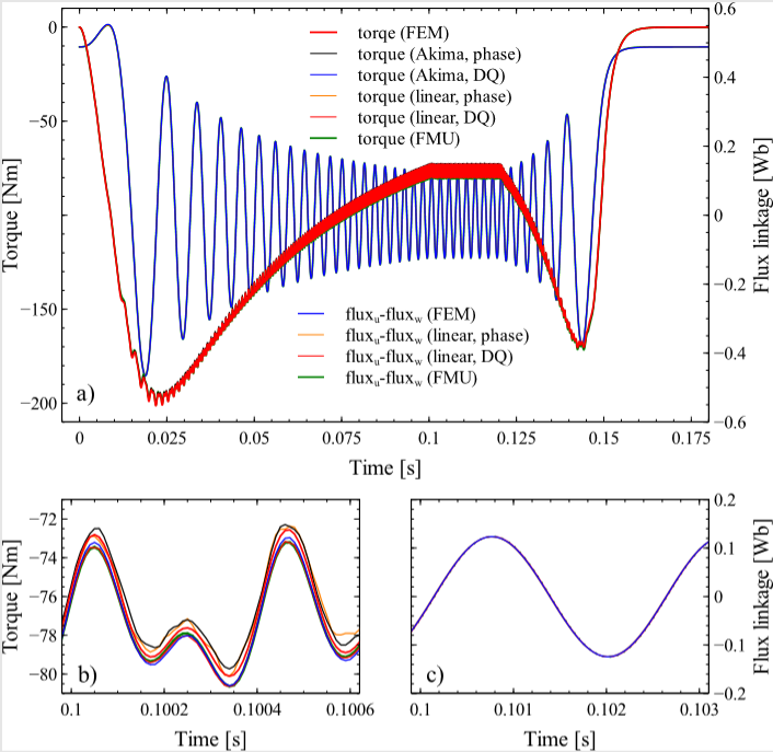
One sees in Fig 3a, which shows the complete timeline, that all approaches yield results quite similar to each other. So all of them seem to work reasonable well. However, if one looks at the magnified cutout Fig. 3b and 3c for torque and ψuw respectively, one can observe small differences in magnitude (in the order of 0.7% with respect to the FEM result) and, especially in the case of the interpolations based on phase quantities (black and orange dashed-dotted curves), somewhat distorted curve shapes for the torque. The distortion is more pronounced in the case of linear interpolation as expected. However, when the interpolation is performed in the DQ-coordinate frame both linear and spline interpolation give rather similar torques. A difference in the compared flux linkage quantity ψuw can hardly been seen even when magnified.
Interesting is also a comparison of the execution times for the different ROM approaches.
Approach abs. runtime [s] rel. runtime [%]
Phase, linear 1.44 50
Phase, Akima 7.32 254
DQ, linear 0.814 28
DQ, Akima 5.61 195
FMU 2.88 100
FEM 14000 486111
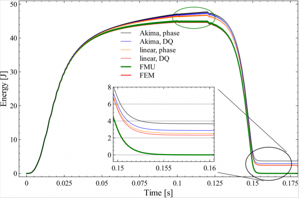
All system analyses have been performed with the variable step size DASSL integration method (default method in Dymola) with an accuracy set to 10-8 and an output step size of 10 μs. The FEM analysis was performed with constant step size forward Euler method with the step size of 10 μs. Last but not least the various methods can be distinguished by their energy conserving behavior. To compare this the total energy given by ∫0t(Pgap (t’) – Pm(t’)) dt‘, where Pgap = Iu ⋅ (dψuw)/dt + Iv ⋅ (dψvw)/dt is the instantaneous power in the magnetic field and Pm = T⋅ ω the mechanical power, is shown in Fig. 4. Energy conservation holds if (i) in the region of constant speed (green ellipse in Fig. 4) the average of total energy over a period stays constant and (ii) the total energy comes back to its initial value when the speed approaches 0. Looking at the results reveal that only the FMU approach and the FEM results are strictly energy conserving. All the flux, torque interpolation approaches in contrast violate this fundamental physical property in the order of 5 to 10%.
Conclusion
Various approaches for ROM creation for PMSM’s were described and compared with each other with regard to accuracy, execution speed and energy conservation. It was demonstrated that the violation of energy conservation resulting from look-up table based methods is not negligible even if the results show only small deviation compared with FEM. To fulfil energy conservation one has to incorporate this property in the interpolation of the vector-valued function f(Id,, Iq, θ) = (ψd,, ψq, T).
Literature
[1] https://www.3ds.com/products-services/simulia/products/cst-studio-suite
[2] https://www.3ds.com/products-services/catia/products/dymola
[3] Gieras, J. F.: “Permanent Magnet Motor Technology”, CRC Press, 2009
We hope you enjoyed this post and have learned about reduced order model approaches to electric machines. If you would like to learn more about this topic, or about anything regarding electromagnetic simulation, visit the SIMULIA Community.
SIMULIA offers an advanced simulation product portfolio, including Abaqus, Isight, fe-safe, Tosca, Simpoe-Mold, SIMPACK, CST Studio Suite, XFlow, PowerFLOW and more. The SIMULIA Community is the place to find the latest resources for SIMULIA software and to collaborate with other users. The key that unlocks the door of innovative thinking and knowledge building, the SIMULIA Community provides you with the tools you need to expand your knowledge, whenever and wherever.

Christian Kremers received his diploma degree in physics from the University of Bonn in 2006. During his PhD at the IHCT (institute for high-frequency and communication technology) at the University of Wuppertal he worked on theoretical and numerical aspects of light matter interaction of nanostructured materials. In 2011 he received his PhD degree in electrical engineering. Afterwards he worked as a researcher at the IHCT. His research interests included the physical modelling of charge carrier movements in CMOS technology at THz frequencies. In 2013 he started his career as an Application Engineer at CST AG. Since the acquisition of CST AG by Dassault Systèmes in 2016 he is strongly involved in the product planning of the low frequency electromagnetic portfolio with a special focus on the electromagnetic simulation of electrical machines.