Anisotropic Polypropylene Calibration: Elastic-Plastic

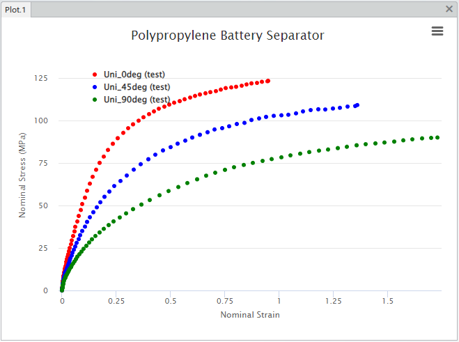
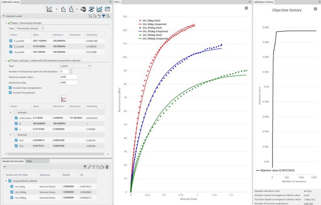
There are many papers and books that discuss the morphology (microstructure) of polymers & plastics. Understanding the morphology may help in understanding the mechanical behavior.  Both the nature of the polymer’s chemistry and the manufacturing process(es) will generally effect the resulting morphology.  The test data above shows uniaxial tension testing on samples taken from a sheet of a polypropylene material.  The 0 degree direction is aligned with what is called the Machine Direction (MD) for the sheet manufacturing process.  The 90 degree direction data is from a sample cut from the sheet at 90 degrees to the MD, often called TD (Transverse Direction).   All of this testing was performed in the plane of the sheet.  We have no data for the through-thickness direction.  This testing is from room temperature.

Polymers & plastics generally have quite a complex mixture of mechanical behaviors, they tend to exhibit both viscous and plasticity (permanent set) behavior.  In this case the polymer also exhibits anisotropic behavior.  Often the engineering challenge is to decide on what material behavior is most important to the application at hand.  For the Abaqus user, this equates to making a decision about the target material model to use in representing the material in the simulation.  In this case, we decide that the viscous behavior (rate effects, stress relaxation, creep) is not important for the application and choose to model the material as elastic-plastic.  Both the elastic part and the plastic part will be modeled as anisotropic.

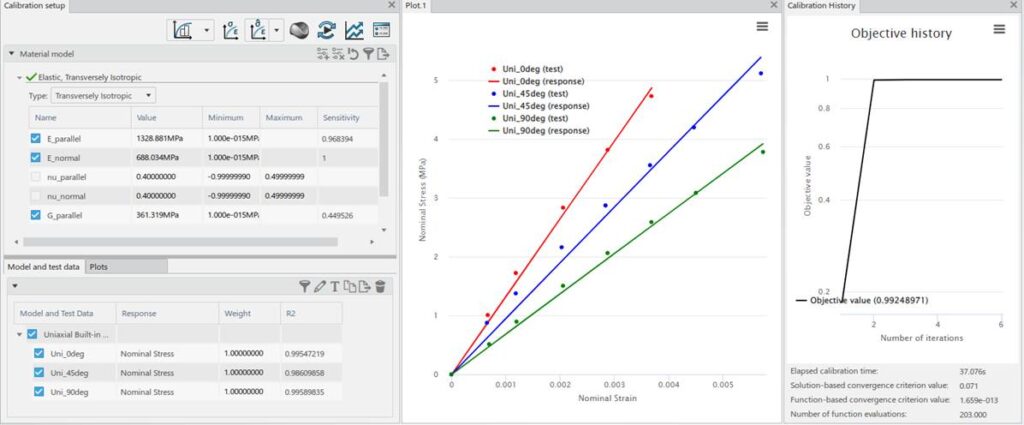
Starting more from scratch…  It is often useful to calibrate in a step-by-step fashion.  Starting from just the test data, truncate all 3 datasets to ~4-5MPa and calibrate a transversely isotropic elastic model to this small strain data.  Set Poisson’s ratios to 0.4 because it is a polymer (we have no test data to determine Poisson’s ratio). 

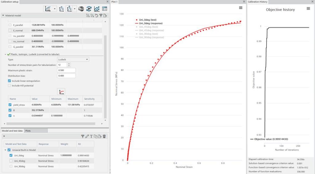
Now go back and “undo” the test data truncation.  Using just the 0 degree data, calibrate an elastic-plastic model (previous elastic part Is reused).  No *Potential use at this point.  I am not a fan of calibrating tabular hardening curves, so I try a few of the analytical forms and Ludwik seems to work pretty well.

Ludwik is a power-law like Johnson-Cook, but ends up as tabular in the solver.  I did not use Johnson-Cook because it cannot be used with *Potential in Abaqus/Standard. 

Add in Hill’s potential, make only these parameters active.  Calibrate to all 3 datasets.  Here I have allowed only the R parameters to vary, not so great result.

Note that there is not enough data to guide R13, R23 or R33.

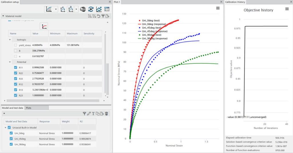
Now, add back in design variables for elastic + plastic + potential: This material model result is attached as a .inp snippet.

Try this out for yourself in the SIMULIA Community by downloading the zip file containing the material model snippet, here.

Interested in the latest in simulation? Looking for advice and best practices? Want to discuss simulation with fellow users and Dassault Systèmes experts? The SIMULIA Community is the place to find the latest resources for SIMULIA software and to collaborate with other users. The key that unlocks the door of innovative thinking and knowledge building, the SIMULIA Community provides you with the tools you need to expand your knowledge, whenever and wherever.