It’s the month of love and what better way to celebrate than with our friend and guest blogger Rob Hurlston from Fidelis! In honor of Valentine’s Day, he’s using ductile damage and explicit analysis to find out what happens to the heart after Cupid’s arrow hits. Uncontrollable desire? Or total damage? Let’s find out!
And stay tuned for more fun tutorials from Rob and Fidelis!
It’s Valentines Day on February 14th, and whether you have that special someone or not, Fidelis is here to spread some love in the form of a ductile damage tutorial video. Having your heart struck by Cupid’s arrow has long been thought to result in being filled with uncontrollable desire, but what about the damage mechanics??? Read on to learn more!

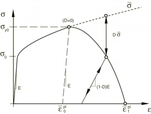
We did a bit of research and it turns out an arrow shot by a bow typically travels at around 150mph or close to 70m/s. That’s pretty fast, but nothing Abaqus’ explicit solver can’t handle! We took advantage of the ductile damage feature to model the impact and ultimate tearing of the heart. Typically, this methodology might be reserved to predict failure in metallic components of a car or airplane, but a little creative tuning of the parameters allowed us to generate reasonably true-to-life behavior of the classic pumpkin drop. For some background, the ductile damage method allows us to prescribe a reduction in both yield strength, Dσ, and elasticity, (1-D)E, as strain increases beyond a predefined threshold (see figure). Eventually, the element reaches zero load carrying capability and is effectively removed from the analysis.
The full workflow tutorial to replicate this analysis within the Abaqus CAE graphical user interface (GUI) is included in this video, but we’ll summarize the important parts here in the order that they were executed:
Parts and Assembly
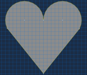
As always, we’ll need to create some parts within the Abaqus CAE GUI. We’ll start with the heart, which will be a shell part and should end up being 400mm in width – we’ve got big hearts over here at Fidelis! This can be drawn in the sketch tool with two semi-circles and tangential lines to meet at the base.
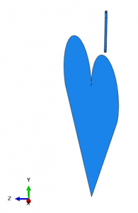
The solid extruded arrow takes a little more effort but should be around 300mm in length, 5mm square, and have a tip and a tail. Check out the video to learn how to do this one.
Once we’ve sketched and extruded the arrow, we can partition it to allow the wood and steel materials to be assigned respectively. To assemble the parts, use the Translate and Rotate Instance operations within the Assembly module. The ‘aim’ is to have the arrow aiming for the location in the heart you intend it to strike and parallel to one of the axis. It’s easier to rotate the heart than the arrow when it comes to applying an in initial velocity later.
Property
The properties of the heart are essentially fabricated, but represent a soft, thin (2mm) shell that can be easily penetrated by the arrow. The wood and steel materials are taken from relevant literature.
Heart Densitly: 1×10⁻¹⁰ tonne/mm3
Heart Elastic: Young’s Modulus = 10MPa, Poisson’s Ratio = 0.3
Heart Plastic:
Yield Stress (MPa) Plastic Strain
1 0
1.5 0.01
2 0.05
2.5 0.1
Heart Ductile Damage: Fracture Strain = 1×10⁻⁵, Stress Triaxiality = 0, Strain Rate = 0
Heart Damage Evolution: Type = Displacement, Softening = Linear, Degradation = Maximum, Displacement at Failure = 5×10⁻⁵ mm
Wood Density: 1×10⁻¹⁰ tonne/mm3
Wood Elastic: Young’s Modulus = 10,000MPa, Poisson’s Ratio = 0.3
Steel Density: 8×10⁻⁹ tonne/mm3
Steel Elastic: Young’s Modulus = 200,000MPa, Poisson’s Ratio = 0.3
Step
This is a simple, single-step analysis in which the arrow is given an initial velocity and then we allow it to fly towards the heart. Since the arrow is traveling so fast, we can run the entire analysis in just 0.02 seconds. The target time increment should be set to 1×10⁻⁶ s for the purpose of any mass scaling that is allowed and we also like to output field data 100 times per step in evenly spaced increments, just so the resolution of the video is acceptable.
Interaction
Again, given the simplicity of this analysis, all we need to apply in terms of interactions is General Contact to the entire assembly – and don’t worry about contact parameters, the Abaqus defaults are fine for this analysis.
Load
As discussed earlier, the arrow will be traveling at 70m/s or 70,000mm/s in this case in the positive x-direction. All we need to do, then, is prescribe an initial condition (Predefined Field) to the arrow.
It’s not just ‘loading’ that is defined within the Load module of CAE. Boundary Conditions also need to be specified here, and in this case, we need an Encastre condition on the perimeter of the heart such that it won’t fly away when it is struck.
Mesh
Most of the parts can simply be meshed using Abaqus default settings. We do want to use the Assign Mesh Controls feature to seed the heart with mesh of ~10mm and the heart with a mesh size of 5mm. This ensures that we get enough fidelity when the element deletion occurs in the heart shells.
Run The Analysis
At this point, we’re ready to launch the analysis (remember to activate the STATUS Field Output so that the spent elements are removed from the visualization!). Hopefully you’ll find this ‘heart warming’ tutorial fun and also see it as a somewhat helpful learning opportunity. The simulation doesn’t take too much time at all to run, so why not play with some of the parameters and initial positions of the parts.

As a provider of all of SIMULIA’s simulation products, as well as a CAE services provider that puts them to good use, we’d love to hear from you about your software and simulation needs!

Robert Hurlston, EngD, PGDip, MEng
Principal and Chief Engineer
Rob is co-founder of Fidelis. Throughout his career, he has worked on and led on a diverse array of projects across a range of industries. This has allowed him to sharpen his analytical proficiency, particularly in the fields of linear and nonlinear stress analysis, dynamics, fatigue, and optimization.
Rob has a strong background in materials, with a specialty in metallurgy and structural integrity engineering. His industrially based doctorate and subsequent post-docs in nuclear materials engineering saw him accumulate over a decade of real-world experience in collaboration with Serco, the University of Manchester (UK), and their partners. Rob has presented much of his work at a number of prestigious international conferences and has also published several journal papers.
Rob holds a first-class master’s degree in materials science and engineering and a postgraduate diploma in enterprise management, along with his doctorate, all of which were completed at the University of Manchester. He is a big soccer fan and an avid golfer. He also enjoys skiing, hiking, and playing the guitar, as well as spending time with his family.
SIMULIA offers an advanced simulation product portfolio, including Abaqus, Isight, fe-safe, Tosca, Simpoe-Mold, SIMPACK, CST Studio Suite, XFlow, PowerFLOW and more. The SIMULIA Community is the place to find the latest resources for SIMULIA software and to collaborate with other users. The key that unlocks the door of innovative thinking and knowledge building, the SIMULIA Community provides you with the tools you need to expand your knowledge, whenever and wherever.

Katie is the Editor of the SIMULIA blog, an expert in engineering and scientific communication, and a strategic digital marketer. Katie has a BA in English and Writing from the University of Rhode Island and a MS in Technical Communication from Northeastern University. She is also a proud SIMULIA advocate, passionate about democratizing simulation for all audiences. Katie is a native Rhode Islander who lives just outside of her favorite city, Providence. She is a true New Englander and loves sharing all the cool things NE has to offer. She enjoys a variety of hobbies including history, astronomy, science/technology, science fiction, true crime, fashion and anything associated with nature and the outdoors. She is also mom to a 6-year old budding engineer and two crazy rescue pups.