3D EM and Circuit Co-Simulation of a DC-DC Converter with Partially Saturated Magnetic Material

Background

The 3D EM and circuit co-simulation of a switching mode power supply, such as a DC-DC converter, involves a 3D model and a circuit model. The 3D model is simulated with CST Microwave Studio (CST MWS) and the components, typically in SPICE format, are connected with the 3D model inside the circuit schematic, CST Design Studio. This approach provides an accurate system response, but the field distribution can’t be correctly modeled using the SPICE. Especially, to model the magnetic field distribution of the inductor that can only be modeled using a 3D inductor model.

In addition, when the output current of the DCDC converter increases, the current at the inductor also increases. The further increment of the DC current at the inductor will lead to (partial) magnetic saturation and results in the decrease of the inductance value.

3D EM and Circuit Co-simulation

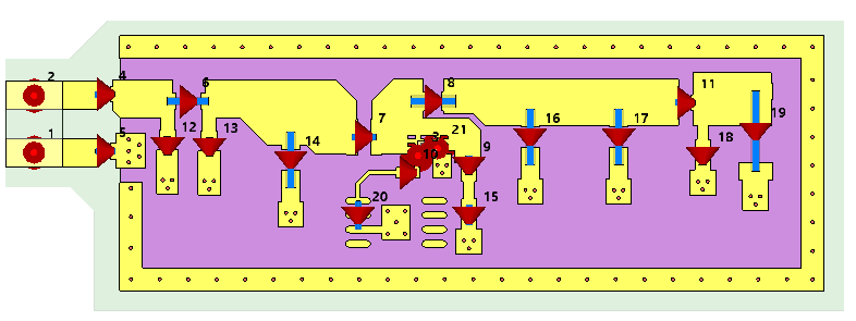
The first step for co-simulation is to import the 3D model of the PCB into CST MWS. The component connections are modeled using discrete ports. Each of the discrete ports is excited and the S-parameter results are available after the 3D simulation. Figure 1 shows the PCB model and the discrete ports.

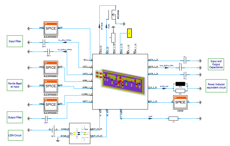
After that, the circuit components such as R, L, C, diode and transistor are connected in the schematic with the CST MWS block, which contains the PCB parasitic information. The electric behavior of the passive circuit components can be represented either using a SPICE model or a touchstone model. For the active circuit components, a SPICE model is required. The complete connection of the circuit components and the CST MWS block can be seen in Figure 2.

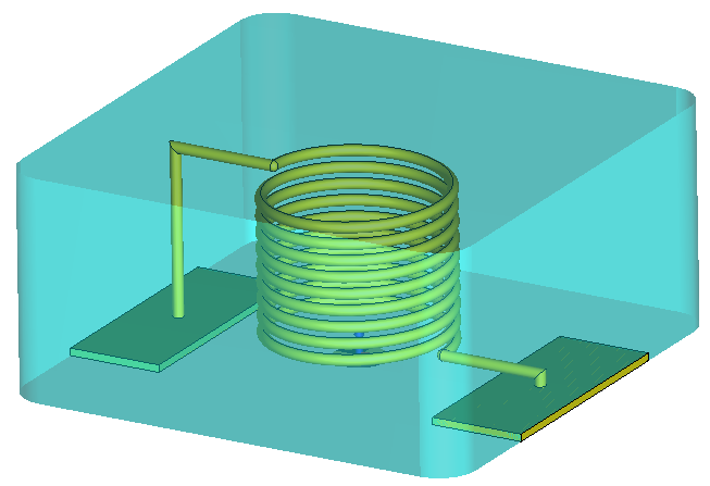
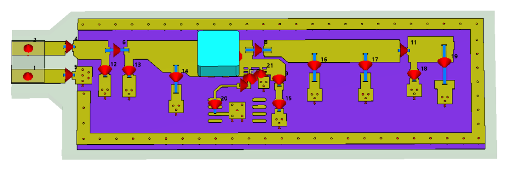
As mentioned earlier, to accurately model the field radiation of the power inductor in the simulation, the 3D model of the coil must be considered. The material of the inductor body is modeled using the Debye 1^st-order magnetic dispersion model with a static permeability of 125. Figure 3 shows the 3D model of the power inductor inside CST MWS. After that, it is placed on the PCB using the import subproject feature as shown in Figure 4 and then simulated.

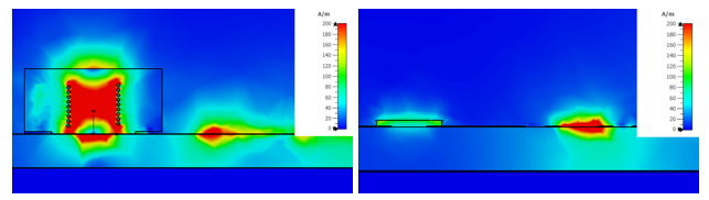
To visualize the difference in the magnetic field radiation, we compare the magnetic field plot of the circuit modeling of the power inductor with a discrete port to the 3D inductor model (Figure 5).

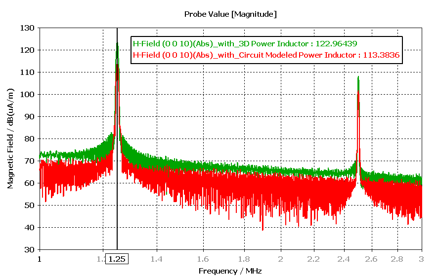
Similarly, we can also observe the magnetic field strength differences using the near-field probe. In contrast to the near-field monitor, the near-field probe provides a wideband result. The probe is placed 10 mm above the PCB. Figure 6 shows an H-field comparison between the 3D inductor model and the circuit-modeled power inductor.

Measuring the magnetic field strength further away from the PCB shows almost no difference between the two approaches. The blue regions, as illustrated in Figure 5, denote the areas where the magnetic field strength becomes less pronounced as we move further away from the PCB.

Modeling of Partially Saturated Magnetic Material

In practical applications for boost converters, when power inductors are subjected to high DC input currents, the magnetic material reaches a state of saturation, which leads to a change in its relative permeability.

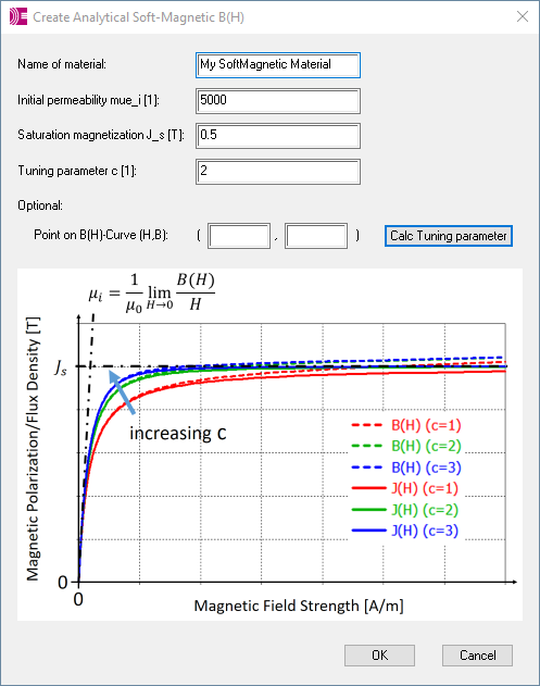
The saturation effect of the magnetic material in the simulation is described with the non-linear behavior of the initial magnetization B-H curve. The B-H curve information can be obtained either from the component vendor or it is described using an analytical formulation. In this blog, we use the material definition with the analytical formulation, which is accessible in CST Studio Suite under VBA Macros –> Materials –> Create Analytical Soft-Magnetic B (H). The interface of this macro is illustrated in Figure 7.

This macro is only visible in a low-frequency CST Studio Suite project. Therefore, make sure to switch to the low-frequency project type if your current CST Studio Suite project is of a high-frequency (HF) type.

The initial permeability, the saturation magnetization and the tuning parameter values are the main material input definitions, and they are automatically created as parameters and listed in the parameter list window. The tuning parameter value controls the slope of the B-H curve in the saturation region and, by default, the value is two. If a known point of the B-H curve is used, the tuning parameter value is automatically calculated based on it.

For this particular example, the initial permeability is 125. As no further material information is available, the tuning parameter and saturation magnetization are initially defined with their default value. These two parameters are tuned based on the DC saturation current information from the vendor’s datasheet, which leads to a 20% reduction of the initial inductance value. The inductance value is evaluated using the magneto-static (MS) solver. The MS solver calculates both inductance values, the apparent- and incremental inductance matrix. Because of the non-linearity of the magnetic material, the inductance value is obtained from the incremental inductance matrix.

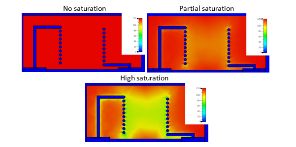
In Figure 8, we illustrate three different spatial distributions of the permeability at the inductor body. First, with low DC current amplitude, without saturation, we can clearly see that the initial permeability is homogenously distributed over the inductor body. As the DC current increases, in this example to approximately 2.8 A, the magnetic material is partially saturated and we can observe the reduction of the permeability mainly at the center of the coil. If we now further increase the DC current, in this case to approximately 8A, the magnetic material saturation increases and the inductance decreases by 50% of its initial value. The permeability inside the coil is now considerably reduced.   

Simulation Workflow to Consider the Saturation Effect

The simulation workflow can be described in the following steps:

• Modeling of the inductor soft magnetic material with the non-linear behavior BH curve. (See the previous section)
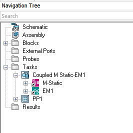
• Creating a simulation project using “Biased Ferrite-EM coupling” in CST Design Studio. This creates automatically two coupled simulation projects, M-static and EM1 (see Figure 9).  
  • The M-Static project calculates the biasing field around the 3D inductor model using the MS solver. The fields are automatically exported to the EM1 project.   
  • The EM1 project is a high-frequency project, which consists of:
    • PCB model of a DC-DC converter (must be imported manually)
    •  3D inductor model and fields from the M-Static project.  
    • Circuit definition of the converter and transient task simulation for co-simulation.

For the M-static simulation, the DC current is defined as excitation. This DC current corresponds to the input current of the boost converter and it can be approximated with the following equation:

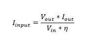
η is the converter efficiency, which can be assumed 90%. The input- and output voltage, as well as the output current, are the converter operating parameters. For this example, the boost converter operates with an input voltage of 12 V and delivers an output voltage of 19 V. The output of the converter is connected to a 12-ohm resistor, representing a static load, which results in an output current of around 1.6 A. The switching frequency is fixed at 1.25 MHz with 35% duty cycle.

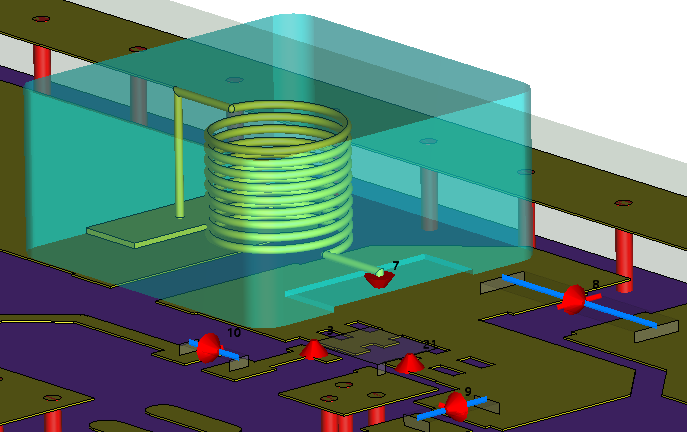
For the high-frequency simulation, EM1 project, the 3d PCB model is imported from the ODB++ layout format. After that, the 3D inductor model is placed on the PCB. The other end of the inductor is connected to the port (in this example number 7). This connection is not necessary but very useful because we can monitor the switching voltage and current through this inductor. The connection of the inductor with the PCB is shown in Figure 10.

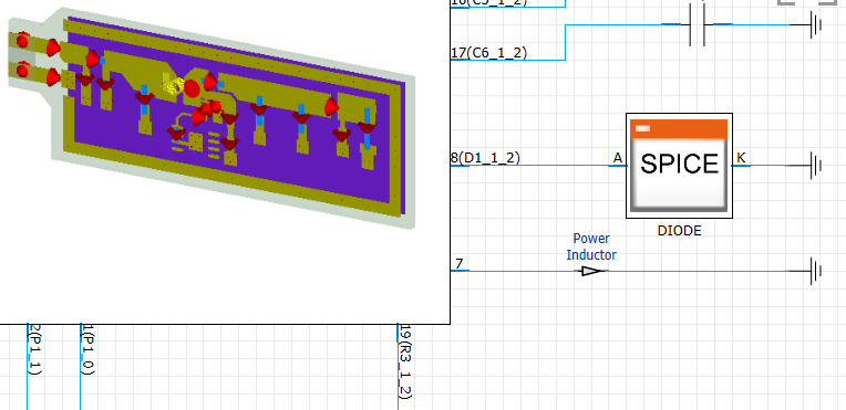
To perform the co-simulation, the circuit connections are to be defined in the schematic of the EM1 project. The circuit schematic connection is similar to the one shown in Figure 2 but without the presence of the inductor SPICE model. This is obvious, because the inductor now has been modeled with 3D model. The port number 7 is directly shorted with the GND symbol to establish the electrical connection with the PCB. The probe “Power Inductor” is placed on that connection to record the current and voltage at the inductor. The Figure 11 shows the schematic connection at the pin 7.  

With the transient task simulation, we can now perform the complete system simulation of the converter. In case the load current increases, we must calculate again the input current with the above equation, and repeat the simulation of the M-static- and EM1 project. 

Simulation Results

The switching current at the power inductor can be monitored in CST Design Studio using a probe, as shown in Figure 11. The increase of the DC current flowing into the inductor leads to magnetic material saturation, which reduces the relative permeability of the magnetic material from its initial value, thus reducing the inductance value. As the inductance value decreases, a higher current ripple at the inductor can also be observed. This can be seen in Figure 12, where the current ripple is compared with the case without saturation.

The current ripple is observed for a single period at the switching frequency in steady state. The saturation case is simulated using a 2.8A DC input current.

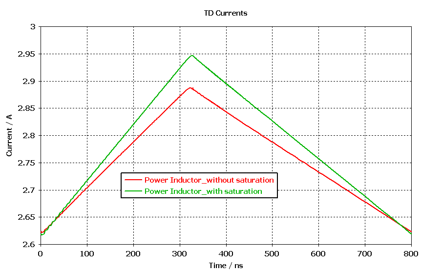
We can see that in the case when the magnetic material has not reached saturation, the observed power inductor current exhibits a ripple with a peak-to-peak of around 265 mA. However, when the magnetic saturation is considered, the observed power inductor current exhibits a ripple with a higher peak-to-peak of approximately 330 mA.

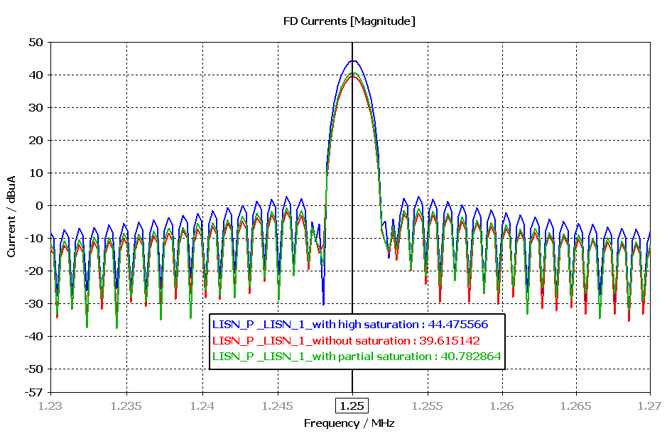
To examine whether the current ripple influences the conducted emission result, we can compare the current spectrum at the Line Impedance Stabilization Network (LISN). This is depicted in Figure 13. We can see that there is only 1 dBmA increment in a partially saturated case (only a 20% reduction of the initial inductance value) and approximately 5dBuA increment for a higher saturation case (for example, 50% reduction of the initial inductance value). This concludes that the saturation effect on the power inductor in this converter example has only a small impact on the conducted emission. Nevertheless, it is important to choose the right inductor with proper current rating to avoid saturation. In addition, it’s important to note that if the saturation effect were considered in the EMI filter components, the impact on EMC performance would become more pronounced.

Conclusion

In this blog, a co-simulation workflow considering the saturation effect of magnetic material on a boost converter has been shown. The workflow is realized by establishing a coupled simulation between the magneto-static solver and the CST MWS frequency domain solver. In the example, the power inductor is subjected to different DC current amplitudes to show the saturation effect. The current ripple at the inductor increases as the power inductor saturates. A similar workflow can be applied to EMI filter components, where the saturation can show more impact on the EMC performance

Interested in the latest in simulation? Looking for advice and best practices? Want to discuss simulation with fellow users and Dassault Systèmes experts? The SIMULIA Community is the place to find the latest resources for SIMULIA software and to collaborate with other users. The key that unlocks the door of innovative thinking and knowledge building, the SIMULIA Community provides you with the tools you need to expand your knowledge, whenever and wherever.