Bring Your Own Model: Deploying a Fine-Tuned ChemBERTa Regressor on the 3DEXPERIENCE Platform

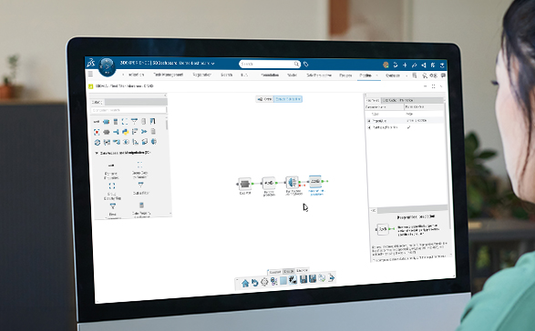
Computational chemists and data scientists can build a robust predictive model in Python in a matter of days or weeks. The harder part is to deploy a model across an organization with a proper lifecycle management and access rights: getting that model in front of the chemists, biologists and lab managers who decide what to make next, in a way that is governed, repeatable and easy to use, and secure.

That is where the 3DEXPERIENCE® platform comes in. With ONNX¹ import in BIOVIA Machine Learning Workbench, a model trained in the framework of your choice becomes a platform asset that can be versioned, published and run in a pipeline. BIOVIA Pipeline Creator applies it to a whole candidate library. BIOVIA Scientific Insight lets scientists review the structures and predictions side by side.

To illustrate the value of this approach, we reproduced the published design workflow with a few nuances to the original scientific paper, where a machine learning model is integrated into a governed, end-to-end drug discovery workflow, from model development and deployment to large-scale candidate screening and scientific review.

Why a Chemical Language Model Matters to Modelers

ChemBERTa² is a transformer that reads a molecule as text: the SMILES string. It is pretrained on a large corpus of SMILES with a masked-language objective, which means it learns to predict hidden pieces of a molecule before it ever sees an assay result. For computational chemists and modelers in life sciences, that has practical consequences:

• Small assays are enough. Fine-tuning adds a small regression layer and trains on your measurements. A screening campaign of around a thousand compounds is a realistic starting point, as in the example below.
• Less feature engineering. The input is the structure itself. There are no physico-chemical descriptors or molecular fingerprints to select and maintain.
• Leverage existing codebase. The model is trained in the Python ecosystem you already use. ONNX is an open format supported by the major frameworks, so models exported from them, such as the transformer in this example, can follow the same deployment path.
• Ranking at scale. Once deployed, the model quickly scores a virtual library in one pipeline run, so the lab starts with the most promising candidates rather than a random sample.

The same pattern applies wherever a structure maps to a property: potency, ADME, toxicity, solubility, or formulation and materials properties.

The Use Case: Ranking Lipids for mRNA Delivery

Lipid nanoparticles carry mRNA medicines into cells, and the ionizable lipid inside them largely decides whether the mRNA is delivered. The space of possible lipids is huge, while the lab can only test so many.

In 2024, the AGILE platform³ addressed this challenge. The researchers measured 1,200 ionizable lipids, trained a Graph Neural Network model on the results, and used it to rank a virtual library of about 12,000 candidates before anything else was synthesized.

Inspired by this use case, we downloaded the pretrained ChemBERTa-77M-MLM model (DeepChem/ChemBERTa-77M-MLM on Hugging Face), fine-tuned it on those 1,200 published measurements (1,100 unique lipids after merging repeats) to predict activity in the HeLa cell line, measured as the log2 fold-change in luciferase signal over untreated cells, and deployed it on the 3DEXPERIENCE platform in three steps.

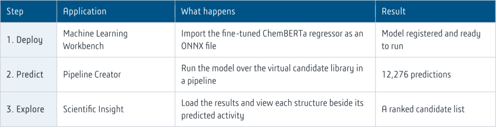
Step 1: Deploy the model in Machine Learning Workbench

We exported the fine-tuned regressor from PyTorch and dropped the .onnx file from 3DDrive. As a preview, the workbench reads the file and shows its metadata and its interface.

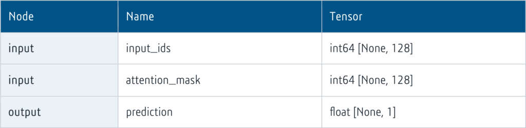
Tokenization happens before import. The ONNX file contains the network only: token IDs and an attention mask go in, one number per molecule comes out. That keeps the contract between the modeler and the platform simple. The first dimension is left open, so the model accepts any number of molecules per call. Once imported, the model appears under Manage Models, with a report listing its inputs and outputs and a menu to publish, export or remove it.

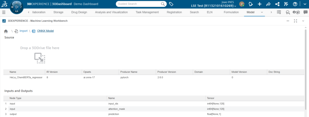
Importing the ONNX model: the workbench lists its metadata and its inputs and outputs.

Step 2: Run it in a Pipeline Creator workflow

We started from the Data Transformation template, which reads a delimited file from the cloud drive, passes the records through an editable subpipeline and writes the result back as a file. The input was the candidate library of 12,276 molecules. Because tokenization is done upstream, each row already holds its SMILES together with the input_ids and attention_mask columns. Inside the subpipeline there are four components:

• Data Port brings the records in.
• Remove prediction removes the prediction property from the incoming records.
• Run Machine Learning Model applies the imported ONNX model to every record.
• Keep smiles, prediction keeps the structure and its predicted value.

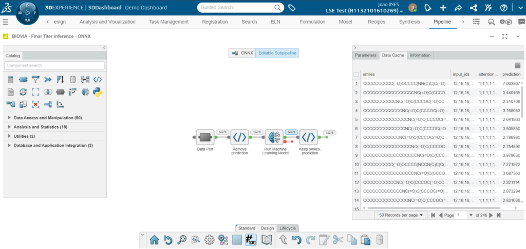
The subpipeline and its data cache: 12,276 records prior to inference.

The pipeline shows the record count at each link and lets you inspect the data after the run. The saved pipeline is reusable: point it at a new candidate library and run it again.

Step 3: Explore the results in Scientific Insight

We imported the output into Scientific Insight, where all 12,276 rows appear with each structure drawn next to its predicted transfection efficiency, expressed as log2 fold-change in luciferase signal over untreated HeLa cells. Sorting by prediction brings the strongest candidates to the top. Both highest predictions share an oleyl (C18) amide tail and a 3-(dibutylamino)propyl head group, a tertiary amine that can pick up a proton in the endosome. They differ in the ester-linked tail, a heptyl heptanoate fragment in the first and a pentyl-nonanoate fragment in the second. This is the pattern we expect from the design rules used to build the library: an ionizable amine head group and tail chains between C10 and C18. As with any ranking, these are model predictions to be tested in the lab.

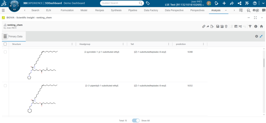
Candidates sorted by predicted activity.

Scientific Insight can also bring in registered substances, formulation data and BIOVIA Generative Therapeutics Design projects from the platform, or any CSV or SD file, so predictions can be analyzed next to the data a team already holds. Bar charts, scatter plots, heatmaps and other chart types help explore how structure relates to predicted activity.

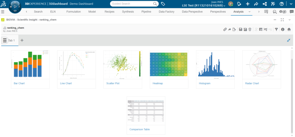
Chart types available in Scientific Insight.

How Well Does It Work, and How Do We Know?

Before trusting a ranking, a modeler wants to know how it was validated. We assessed the approach in a companion study in BIOVIA Pipeline Pilot that fine-tuned the same ChemBERTa model on the same dataset of 1,200 measurements (1,100 unique lipids). This is how it was set up.

• A random 70/15/15 split. 770 molecules for training, 165 for validation (used to stop training early) and 165 held-out for testing, scored once. We chose a random split because it matches how the model is used: ranking new combinations of head groups and tails that are largely built from the same families as the measured lipids. It measures how well the model interpolates within that chemistry.
• Three seeds. The same split was trained three times with different random seeds, so results are reported as a mean and a spread rather than a single lucky run.
• A simple baseline. A random forest on Morgan fingerprints, trained on the same split, shows what a classic method achieves on this dataset.
• Rank-oriented metrics. Alongside R² and RMSE we report Pearson and Spearman correlation, and top-tier precision: lipids are sorted into six tiers, as in the AGILE paper, and we ask how often a lipid predicted in the top tier truly belongs there.

Reading the numbers

• It ranks well. A Spearman correlation of 0.69 and a top-tier precision of 0.51, against 0.17 for random, meaning about half of the lipids it puts in the top tier belong there. In none of the three seeds was a lipid predicted top-tier truly in the bottom tier.
• A simple baseline is strong on a dataset this small. The fingerprint random forest matches the transformer on R². The transformer is modestly ahead on rank correlation. The practical point is that either model class deploys the same way, so you can compare them on your own data.
• Read predictions as a ranking. The models pull values toward the mean. Use percentiles, not the absolute prediction.
• Noise sets a ceiling. Repeat measurements of the same lipid differ by an RMSE of about 1.0 log2 unit, roughly two-fold, so no model can match the assay exactly. The model’s test RMSE is about 2.4.
• Know the limits. A random split does not test extrapolation. This model is a tool for prioritizing within the chemistry it has seen, and the lab remains the final test.

Watch the video to see the complete workflow in action:

Getting Started with Your Own Workflow

For more on the platform, read our earlier posts on Machine Learning Workbench. Pipelines built in Pipeline Creator can also be shared as virtual advisors in Virtual Companion, so scientists can use a model without opening the pipeline. To explore how this could work with your own models, contact us.

References

1. ONNX, the open standard for machine learning interoperability. https://onnx.ai
2. Chithrananda, S., Grand, G. & Ramsundar, B. ChemBERTa: Large-Scale Self-Supervised Pretraining for Molecular Property Prediction. arXiv:2010.09885 (2020).
3. Xu, Y., Ma, S., Cui, H. et al. AGILE platform: a deep learning powered approach to accelerate LNP development for mRNA delivery. Nature Communications 15, 6305 (2024). https://doi.org/10.1038/s41467-024-50619-z