What is Vortex-Induced-Vibration (VIV)?
Vortex-Induced-Vibration (VIV) is a well-known phenomenon caused by the interaction of a fluid flowing over a bluff body. The effect is at its most severe when the flow is perpendicular to the body. As real fluids behave in a viscous manner, a boundary layer forms on the surface of the body and is liable to separate from it forming a vortex, which in turn can alter the pressure distribution on the surface. Generally, these vortices are created non-symmetrically and hence an alternating pressure distribution is established on the surface that tends to promote motion in the body. If the frequency of the vortex shedding coincides with a resonant frequency of the structure, then significant, and potentially harmful, deformations can be created.
Where do Vortex-Induced-Vibrations occur?
VIV can be present at relatively low Reynolds numbers (low speeds) and if the fluid in question is air, can develop into aero-elastic ‘flutter’ at higher speeds. The most dramatic example of this phenomenon was that of the Tacoma Narrows suspension bridge in 1940 (https://en.wikipedia.org/wiki/Tacoma_Narrows_Bridge), which was completely destroyed by a relatively low speed, 40 mph cross-wind travelling down the gorge.
The physics of VIV is well understood, particularly for simple shapes with circular cross-sections. As it happens, structures with circular cross-sections are relatively common in engineering; chimneys, high voltage power cables, tethers, tubular supports, pipelines etc. In many cases, considering the problem of VIV in two-dimensions is an adequate approximation of the physics, but extending the mathematics of VIV to three-dimensions is much more complex and can only be practically done using numerical simulation.
The physical response of a structure of circular cross-section in 2-D has been studied extensively and as long ago as 1878, Czech physicist Vincenz Strouhal proposed an empirical formula that linked the frequency of vortex shedding to the section diameter and bulk flow velocity.

A 3-dimensional numerical simulation of VIV requires two distinct physical systems to be linked; the fluid system which is governed by velocity, viscous shear, pressure and turbulence and the structural system which is governed by compliance, strain and displacement. Moreover, these systems must be solved in the same time frame which means that the numerical analysis must be executed as a co-simulation.
Fluid-Structure-Simulation Set-Up
Numerical co-simulation is a solution technique that is available on the 3DEXPERIENCE platform. Simulating VIV is a fluid-structure interaction (FSI) problem that involves the construction of separate solid and fluid simulation objects that are solved simultaneously, with data being exchanged at specified intervals. In the case of a CFD model (https://www.3ds.com/products-services/simulia/products/fluid-cfd-simulation/) solved using the 3DSFLOW solver, traction vectors are exported to the structural model and displacements and velocities are imported. For the structural model, solved using the Abaqus solver (https://www.3ds.com/products-services/simulia/products/structure-simulation/, the opposite happens with displacements and velocities being exported while traction vectors are imported from the flow solver. The flow of data is controlled through the use of the SIMULIA Co-Simulation Engine (CSE).
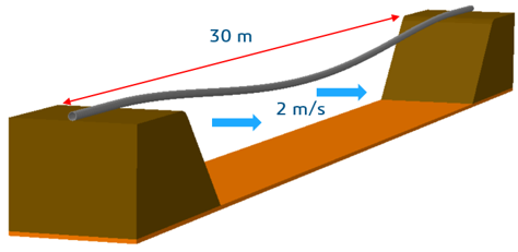
In simulating 3-dimensional VIV, there are three particular challenges that need to be addressed. Suppose, by way of example, we take the case of a 0.2m dia. pipe-line suspended in water that is flowing in a direction perpendicular to the pipe. The pipe itself is grounded at either end of the 30m free span. The fluid and solid models must be co-located.
Meshing of long structures for fluid-structure interaction simulation
Structures susceptible to VIV are characterized by having one dimension much longer than the other two. While this is generally not an issue for the structural model, it does pose problems for the fluid mesh where, in this example, fine discretization is required to represent the boundary layer around the pipe in two-dimensions but a much coarser discretization is desirable in the third dimension in order to reduce element count. For this reason, the Hex Dominant Mesher is not suitable for this application as it attempts to equalize element sizes in all three dimensions.
Mesh extrusion techniques are better suited to this application as the user has more control over the mesh size in all three directions. However, for this to be effective, the flow solver must be able to cope with element aspect ratios of 100-200 to 1 if the element count is to be kept to practical levels.
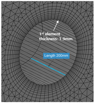
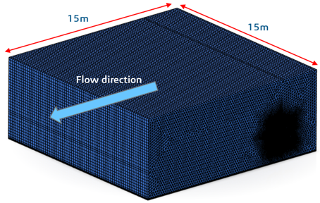
A 2-D surface mesh, using a combination of triangular and quadrilateral elements, is first specified at one end of the full fluid domain in order to get an adequate discretization around the initial location of the pipe. This surface mesh is then used as a template for the 3-D fluid elements that are extruded to populate the fluid. The fluid domain therefore comprises brick and wedge type fluid elements. Before simulation, the surface mesh is declared to be of type ‘construction’ and hence takes no part the in the CFD simulation.
In this example, the model takes advantage of symmetry so the fluid domain need only extend for 15 meters. Even so, the fluid domain contains over 1 million elements.
Mesh motion
For a suspended pipeline subjected to a normal water flow, some oscillation of the pipe will be expected. As 3DSFlow does not allow neither the creation nor elimination of fluid elements, the movement of the pipe has to be accommodated by the original mesh of fluid elements. The 3DSFlow solver achieves this by automatically morphing the fluid mesh at each solution iteration according to some basic guidelines specified by the User. Internally, and completely separate from the fluid solution, the fluid mesh is considered to be made of a crushable foam material that deforms as the pipe-line moves, and the elements deform accordingly as they would in a static finite element simulation. Additional control is made available to the User via a mesh motion dialogue box which enables the local stiffness of the foam to be modified. For example, the foam stiffness adjacent to the pipe can be locally increased such that the boundary layer elements retain their shape as the pipe moves and the mesh morphs.
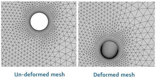
There is obviously a limit to how much pipe movement can be accommodated by this technique before the elements become too distorted for the solution to proceed, but in this example, the motion of the vibrating pipe is captured without a problem.
Coupling of structural and fluids simulation
Two separate solvers are used in the simulation and the solutions of each are coupled through the common interface defined by a ‘port region’. Using two separate solvers in the fluid-structure interaction problem enables the most efficient technology to be used for each physical system. The integrity of the solution relies on the accurate exchange of data through the common interface and different techniques may be employed according to the strength of the coupling.
The coupling strength is influenced by a number of parameters which determine whether the coupling can be classed as weakly, moderately or strongly coupled. Weakly coupled, or one-way coupled systems, can be solved using an explicit coupling scheme where the fluid and solid velocities at the coupling interface generally do not match. This approach works well for simulations where the structure/fluid density ratio is large such as in aero-elastic coupling. However, if the coupling is stronger, as in co-simulations involving liquids, then explicit coupling methods may suffer from instabilities and inaccuracy.
The 2022x FD04 release of 3DEXPERIENCE includes extrapolation methods, accelerators, filtering techniques and convergence criteria to the SIMULIA Co-Simulation Services to provide state of the art co-simulation capabilities for implicit-iterative coupling. In particular, the Quasi-Newton accelerators increase the radius of convergence from a stability point of view, allowing us to tackle stronger coupled physics and reducing the computation effort by reducing the number of coupling iterations required to attain certain convergence criteria. Furthermore, they allow us to tackle strongly-coupled physics problems, which we were not able to solve previously. Our VIV pipe-line example is one such, moderately coupled, problem that benefits from these implicit coupling methods.
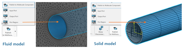
The port region defines the interface through which data will be exchanged during the co-simulation. The port region for the solid and fluid models must be geometrically co-located.
Fluid-Structure Co-simulation set-up
Pipe structural simulation
The pipe structural model consists of a single layer of C3D8I incompatible mode elements with a kinematic coupling connected to a central reference point at either end. At one end the reference point is completely fixed and at the other end symmetry boundary conditions are specified.
The analysis procedure used is implicit dynamic using a fixed time increment of 0.01 seconds.
Water CFD model
The fluid domain representing the water consists of predominantly 6 node F3D6 elements with 8 node F3D8 elements surrounding the pipe. An inlet boundary condition has a normal velocity of 2 m/s specified with a pressure boundary that matches the hydrostatic pressure gradient at the outlet end of the domain. A symmetry boundary is defined on the symmetry plane and slip wall conditions are defined at the other domain boundaries apart from the sea floor which is specified as no slip.
A transient fluid procedure including a realizable K-Epsilon turbulence model is specified using a fixed time increment of 0.01 seconds.
Co-simulation set-up
An implicit coupling scheme using a Gauss-Seidel algorithm is specified using a fixed data exchange time of 0.01 seconds. The total solution time is 12 seconds.
Run time diagnostics
As the co-simulation is running, the cfd.sta should be available for inspection. This file gives details of the progress of the job and how easy or difficult it is for convergence to be achieved.
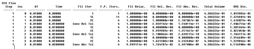
Two measures of iterative convergence are used; one being an absolute value which is appropriate when there is little/no relative movement between the fluid and the structure, and another being a relative value which is used when the structure has some significant velocity. These convergence values have defaults which may be overridden by the User depending on the nature of the co-simulation. The software enforces a minimum of three external iterations irrespective of the value of convergence achieved.
Fluid-Structure Co-simulation Results
The results from the co-simulation are both qualitative and quantitative; the former are typically velocity/vorticity/pressure contours in the water combined with displacements of the pipe, and the latter takes the form of time-displacement XY plots at various locations on the pipe. This gives a measure of both the amplitude and frequency of vibration of the pipe.
The structural model results also contain a full set of stress, strain and displacement results for the pipe which may be used to assess structural integrity and fatigue performance.
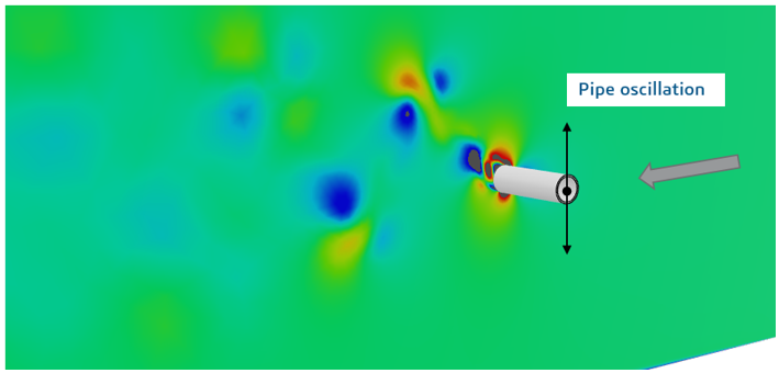
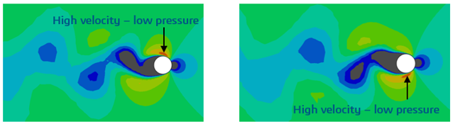
The illustration shows the contour of velocity in the water combined with deformation of the pipe at the end of the 12 second simulation. The formation of vortices and the pattern of shedding from the pipe can clearly be seen. The picture shows the state of the model just inboard of the symmetry plane, and this pattern is repeated to a greater or lesser extent at all locations along the pipe-line.
Assuming a Strouhal no. of 0.2, the frequency of vortex shedding from the pipe can be calculated as: 0.2 x v/d =0.2 x 2.0/0.2 = 2Hz.
If the cylinder itself oscillates, the vortices are shed at or near points of maximum displacement and therefore the width of the wake is increased. As a consequence the pressure drag is increased together with the lateral force, and the frequency of vibration is decreased.
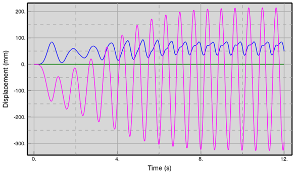
The XY graph above shows the cross-flow (pink) and in-line (blue) amplitude of displacement for the pipe at the location of the symmetry plane. By inspection, the frequency of vibration is approximately 1.5Hz, and this value is in accordance with the prediction of reduced frequency as a result of pipe oscillation. When the oscillation has reached a ‘steady-state’, the peak-to-peak displacement of the pipe is approximately 500mm, which may be expressed as 2.5D in terms of the cylinder diameter.
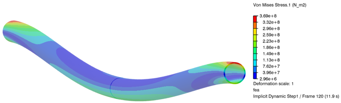
With regard to the structural analysis, the SIM file can be post-processed separately or in conjunction with the CFD results. The figure shows the distribution of Von Mises stress in the pipe at t=11.9 seconds (figure shows results mirrored about the symmetry plane). Stress or strain values in the pipe can be used with the frequency of vibration to assess fatigue performance if necessary.
Summary
The 3DEXPERIENCE platform can be used to perform complex coupled co-simulations such as Vortex-Induced-Vibration on pipe-lines. The 3DSFlow solver is available via the FMK role and the non-linear structural dynamic analysis with Abaqus is available via the SYE role.
The interaction between the fluid and structural physics is controlled through the SIMULIA Co-Simulation Engine which provides advanced coupling algorithms that help achieve accurate converged solutions in an efficient manner. The same technology illustrated here can be used to investigate other Fluid-Structure-Interaction problems such as blood flow in arteries, peristaltic pumps and bottle-squeeze type applications.
For further discussion and illustrations of simulating VIV using the 3DEXPERIENCE platform, an eSeminar has been scheduled for 7th December 2022.

SIMULIA offers an advanced simulation product portfolio, including Abaqus, Isight, fe-safe, Tosca, Simpoe-Mold, SIMPACK, CST Studio Suite, XFlow, PowerFLOW, and more. The SIMULIA Community is the place to find the latest resources for SIMULIA software and to collaborate with other users. The key that unlocks the door of innovative thinking and knowledge building, the SIMULIA Community provides you with the tools you need to expand your knowledge, whenever and wherever.

Stephen King is a SIMULIA Structures Industry Process Senior Consultant.