Where Does EMC Simulation Fit in Electric Vehicle Development?
It fits at every stage, from the first enclosure sketch to the assembled system. That was the case made across a three-part SIMULIA® webinar series in June and July 2025. Each talk covered one stage of development, set up a realistic electric vehicle (EV) problem in CST Studio Suite and showed what simulation can tell an engineering team before hardware exists.
If you’re short on time and can’t watch all three webinars right now, here is what each session covered and the numbers that matter.
| Stage | Talk | Question it answers | Headline result |
| Early: risk assessment | Shielding effectiveness | How much will this enclosure protect what’s inside it? | A reverberation-chamber workflow matched a 50-run plane-wave sweep with only 8 simulations |
| Middle: component design | High-voltage filter design | What is the smallest, cheapest filter that passes CISPR 25? | Circuit models alone were far too optimistic above about 20 MHz; adding 3D busbar parasitics changed the design |
| Late: system validation | Automotive Ethernet emission and high-voltage/low-voltage coupling in a battery pack | Which part of the assembled system is the weakest link? | Fixing the cable connector gave a 20 dB improvement; improving the connector cut coupled emission peaks by about 80 dB |
Talk 1: What Determines an Enclosure’s Shielding Effectiveness?
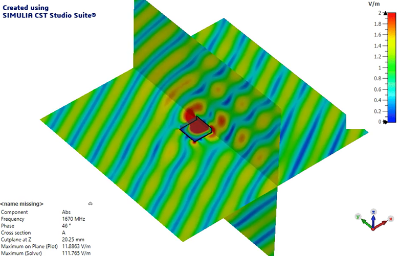
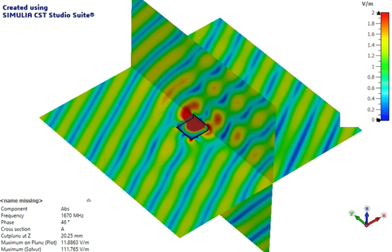
Shielding effectiveness is not a single number. It depends on the source, the type of field (electric or magnetic) and where you measure. The first talk made that point with a sequence of models, from a flat copper plate to a full EV battery pack.
Theory and simulation agree when you compare like with like. Textbook equations assume an infinite plane wave incident on an infinite shield, measured directly at the surface. When the simulation probe was 1 µm from the plate, the results closely matched the equations. At 100 mm, standing waves and edge effects pulled them apart. Neither result is wrong; they answer different questions.
Empty enclosures can amplify fields. A sample enclosure gave roughly 35 dB of shielding at 200 MHz. Near 1 GHz, internal resonances pushed shielding below zero, meaning the field inside was stronger than outside. Adding a lossy block the size of a PCB shifted the resonance and largely removed the negative band.
A faster way to model a reverberation chamber. Sweeping a plane wave over 25 incidence angles, with and without the enclosure, took 50 simulations. A new workflow generates a small set of field sources that reproduce a reverberation chamber’s random, all-direction field. Four sources met the chamber’s 3 dB uniformity criterion, so the same answer was obtained after 8 runs. The workflow arrived as a preview in a 2025 service pack. Fuller automation was released in 2026 with documentation in the knowledge base. The 2027 release of CST Studio Suite will also bring more updates.
Applied to a battery pack. The team pre-meshed a full underbody battery pack on the 3DEXPERIENCE® platform and asked whether low-frequency magnetic fields from the inverter would reach the passenger compartment. With a realistic inverter spectrum, the field remained below the ICNIRP human exposure limit for a 0.9-mm steel lid. A second study checked how many screws the lid needs. Using the switching signal’s envelope instead of a full switched simulation cut run time from about 30 minutes to a few seconds, with close agreement.
Talk 2: How Do You Design a High-voltage EMI Filter with Simulation?
Start with a fast circuit model, then add physical detail only where it changes the answer. The second talk walked through a one-stage filter for a 400 V, 200 A inverter, aiming to pass CISPR 25 Class 1 in the smallest, lowest-cost package. The same method applies to small motors in pumps or household appliances.
Model the noise source as an envelope. The inverter’s switching noise was represented by its spectral envelope (10 kHz switching, 100 ns rise time) rather than a full switched waveform. Every real switching signal falls within that envelope, so it gives a fast worst-case.
Explore the design space at circuit level. A 27-run parameter sweep of a pi filter took under a second per run. An optimizer then proposed component values, rounded to purchasable parts: 20 nF and 50 nF capacitors and a 50 µH inductor.
Then add the 3D parasitics. Connecting the circuit to a 3D model of the busbars and housing told a different story. The two models agreed up to about 1 MHz and stayed close to 10 MHz. Above about 20 MHz, the circuit-only model was far too optimistic.
Design out mounting sensitivity. Filter performance changed with the length of the grounding strap, which depends on how the unit is installed in the vehicle. A shielded cable between housing and measurement point removed that dependence and fixed the design at its worst case.
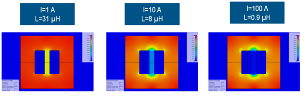
Get the ferrite right. At 100 A, an ungapped core saturated and its inductance fell from 31 µH to 0.9 µH. A 0.5 mm air gap held the variation between 1 A and 100 A to 3.6%. A simple physical (Debye) model of the ferrite’s frequency response proved more reliable than band-limited vendor measurements.
Fix problems with the cheapest part. The realistic inductor model removed the high-frequency problem predicted by the circuit model, but exposed a differential-mode resonance. Raising the CX capacitor value addressed it at lower cost than a larger core, and the housing could be shortened.
A final check with the full switched inverter matched the envelope-based trends. Every simulation ran in minutes on a strong laptop.
Talk 3: How Does Simulation Find the Weak Link in an Assembled System?
By adding and removing parts of the system one at a time and measuring the change in emission. The third talk applied that approach to two cases that often trouble EV programs.
Radiated Emission from an Automotive Ethernet Link
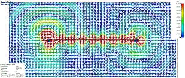
The model consisted of two boards joined by half a meter of twisted-pair cable, running 1 Gbit/s automotive Ethernet. The full 3D model, including cable twists, simulated 0–2 GHz in about 4 hours 40 minutes on a single machine. Emission was evaluated at 3 m from all directions, keeping the worst case at each frequency.
| Change to the design | Effect on radiated emission | What it showed |
| Add a common-mode choke to a well-balanced layout | About 7–8 dB lower, little effect at high frequency | A choke can only filter the common-mode noise that exists upstream of it |
| Introduce trace imbalance after the choke | Choke no longer helps | Place the choke as close to the connector as possible |
| Seal the PCB in a metal box | Only 3–4 dB lower | The cable assembly, not the board, was the main radiator |
| Add a fully shielded cable | About 9 dB lower | The connector, not the shield, was leaking |
| Extend the connector shell for a 360° shield connection | About 20 dB lower at the highest peak | The connector was the weakest link |
| Shield the PCB as well | About 70 dB lower (idealized) | Once the cable was fixed, the board was the remaining source |
Some of these changes would be hard to try on real hardware. In simulation, each was a quick CAD edit.
High-voltage to Low-voltage Coupling in a Battery Pack
Even when high-voltage cables are shielded, low-voltage wiring for the battery management system often is not. Noise from the high-voltage busbars can couple into that wiring and radiate once it leaves the pack. The busbars’ length produced resonances around 10–30 MHz, where coupling peaked.
The talk compared two layouts. Moving the battery management module further from the busbars lowered emission peaks by almost 50 dB. Where the layout can’t change, a simple filter on the low-voltage lines cut the peaks by about 80 dB, bringing the poor layout close to the good one. Each 3D simulation took about 2 hours.
What Do the Three Talks Have in Common?
Four practices came up in every session.
- Start simple, add complexity only when it changes the answer. Circuit models and envelope sources gave fast first answers; 3D detail and full switching came in later, as checks.
- Use worst-case sources to move quickly. Signal envelopes and worst-case-over-direction evaluation yielded conservative results in seconds or minutes rather than hours.
- Think in terms of source, coupling path and sink. Every study separated where the noise starts, how it travels and what it disturbs, then tested changes to each.
- Know your input data. Results are only as good as the capacitor parasitics, ferrite properties and motor impedance behind them. Vendor data and earlier projects are the best sources; reasoned estimates are a valid starting point.
Watch the Webinars
- Talk 1: https://events.3ds.com/simulia-shielding-effectiveness-simulation
- Talk 2: https://events.3ds.com/hv-filter-design-simulation
- Talk 3: https://events.3ds.com/emc-system-level-simulations
If your team is deciding where EMC simulation belongs in your development timeline, start with the white paper.
Frequently asked questions
What is EMC simulation?
Electromagnetic compatibility (EMC) simulation predicts whether an electronic product will emit too much electromagnetic noise or be disturbed by noise from other equipment. It combines circuit models with 3D electromagnetic models, allowing teams to check designs against standards such as CISPR 25 before building prototypes.
Why is EMC harder in electric vehicles?
EV powertrains switch hundreds of volts and amps at high speed, and that switching is a strong noise source. Tight packaging also leaves little room to separate noisy high-voltage parts from sensitive low-voltage electronics.
Is shielding effectiveness a fixed property of an enclosure?
No. It changes with the source, the field type, the measurement position and the enclosure’s contents. Resonances can even make an empty enclosure amplify fields at certain frequencies.
Can a filter be designed with circuit simulation alone?
Only for a first estimate. In the filter talk, the circuit-only model was far too optimistic above about 20 MHz because it left out the parasitics of the busbars and housing.
Where should a common-mode choke go on a PCB?
As close to the connector as possible. A choke can only filter common-mode noise created before it, so any imbalance between the choke and the connector bypasses it.
Why doesn’t a shielded cable always reduce emissions?
Leaks usually happen at the ends, not along the shield. In the Ethernet study, a perfect shield gave about 9 dB of improvement until the connector made a 360° connection to it, which raised the improvement to about 20 dB.
How long do these simulations take?
The filter studies ran in minutes on a laptop. A full 3D battery-pack coupling study took about 2 hours. The detailed twisted-pair Ethernet model took less than 5 hours on a single machine.

Andreas is a senior solution consultant for electromagnetic simulation at Dassault Systèmes in Darmstadt, Germany. After receiving his PhD in numerical electromagnetics from the Darmstadt University of Technology in 2007 he joined CST which later became a part of Dassault Systèmes. His main interest lies in the simulation of electromagnetic compatibility of electronic systems, ranging from high-speed to power electronics.