Debugging Abaqus Models

The following blog was authored by Ritu Singh, a mechanical engineer from Auburn University, Alabama, with six years of experience. She excelled as a senior design engineer for three years before transitioning to a writer and team lead for three years, specializing in creating accessible content. Currently, Ritu serves as an Advocacy Offer Marketing Specialist in Global Marketing at Dassault Systèmes for the SIMULIA brand, where she combines her engineering acumen with her writing skills to craft compelling marketing content.

Introduction

Debugging Abaqus/Standard models can be complex, especially when confronting convergence problems in structural simulation.

This blog focuses on debugging Abaqus models, which refers to fixing convergence problems in Abaqus/Standard. Debugging can refer to a range of things, from building and fixing problems in a mesh to correcting basic modeling mistakes, misspelled keywords, and more. However, this blog aims to learn how to fix convergence problems in Abaqus/ Standard.

Understanding Convergence in Abaqus/Standard vs. Abaqus/Explicit

Abaqus/Standard is the original Abaqus solver code, dating back to the early 1980s. It is a finite element solver code, also known as an implicit solver, with many capabilities. These range from general nonlinear static and dynamic simulations to linear simulations, including linear dynamics, heat transfer, acoustics, piezoelectric effect, and more.

Abaqus/Standard uses an incremental, iterative approach for general simulations. It is built around the Newton-Raphson method, a numerical technique used to target convergence issues, requiring a comprehensive debugging strategy.

This method’s successful completion results in so-called ‘convergence,’ while its failure leads to non-convergence. It is crucial to distinguish between these two states to address non-convergence effectively.

In contrast, Abaqus/Explicit is a dynamic explicit package released around 1992. It is an explicit solver that operates on a fundamentally different solver technology. Abaqus/Explicit has various capabilities such as general nonlinear dynamic simulations, heat transfer, and acoustics coupled with structural, large deformation methods and robust contact algorithms suitable for complicated 3D contact models.

A dynamic explicit analysis package, Abaqus/Explicit, does not use the Newton-Raphson method and, therefore, does not have convergence issues. However, explicit codes can face numerical stability concerns.

Users facing severe convergence problems in Abaqus/Standard can consider switching to Abaqus/Explicit. Since the interface for both the solvers is notably similar, transitioning to Abaqus/Explicit can help mitigate convergence challenges encountered in Abaqus/Standard simulations.

Example: Connector Spring

The first example involves a one-element model with one connector element to which a force is applied. A nonlinear spring stiffness balances the force. The connector element is a Cartesian-Cardan connector. Its first component of relative motion has a nonlinear stiffness, while the other components of relative motion are constrained.

Since the spring is nonlinear in one direction, this model is relatively straightforward and uses a static load step. This means we are going to test how far the spring stretches under the load. It is crucial to identify the critical model features when debugging a convergence issue:

• Connector element with a nonlinear stiffness
• Boundary conditions, including connector motion constraints
• Concentrated loads
• Static procedure.

We must understand the features in the model even if debugging is not required. Understanding how to use the model features is as crucial as understanding the problems they can cause such as,

• Nonlinear springs may have non-monotonic force/deflection behavior
• Multiple constraints might interfere with each other.
• Follower loads may cause the need for the unsymmetric solver.
• The simulated process may be quasi-static, causing the static analysis’s failure.

Knowledge of potential pitfalls is developed through both training and experience. This is true for almost any complicated human endeavor. Through training, one can circumvent relying solely on experiential learning while enhancing one’s ability to identify and address challenges effectively.

In the following example, the model fails to complete as-is. The first thing to do is look at the status file. (You may prefer to use Job Diagnostic in Abaqus/Viewer, but I prefer text files.) The green text indicates a convergence problem.

My log file contained an error code message, but these are lower-level, system-related problems that I would need to investigate separately. Here, we are facing a run-of-the-mill convergence problem. Once we have identified the issue of the analysis abruptly terminating, we must examine the message file.

I prefer to first inspect the end of the file. I like to do this while I have the ODB open in Abaqus/Viewer with the deformed shape of the last saved result displayed. In this case, the message indicates that the required time is less than the minimum specified, which is a generic message.

Often, error messages reiterate what’s already known. When I review the message file, I typically have a picture displayed of the model’s deformed shape just before the error occurred. However, since this is a single-element model, there’s not much to visualize.

Now that I know the excessive cutbacks caused the error, I can backtrack through the message file, noting the critical nodes and elements and locating them in the deformed mesh. I need to identify patterns in the numbers so I ask questions to myself, such as:

• Does the same group of nodes consistently have the largest residuals?
• Does the same group of nodes consistently cause problems with the contact?
• Are the largest corrections at the same few nodes?
• Is the plasticity seemingly out of control in the same group of elements? Etc.

The number patterns can help you identify the region of the mesh that is causing the problem. You can quickly locate these entities within the displayed mesh.

Now, with the job interrupted abruptly; hopefully, you have some intermediate results saved. You must formulate a hypothesis to mitigate the issue. This hypothesis must align with the identified problematic mesh region and potential issues inherent to the model’s features.

You must scrutinize known results through animations or contour plots of stress and displacement to refine this hypothesis. With a working hypothesis, the next step involves modifying the model to address the hypothetical problem.

With luck, once you implement the fix, the issue will be resolved. However, if the problem persists or new complications arise, an incorrect hypothesis could be the cause. In such scenarios, especially when dealing with convergence problems, it is crucial to practice perseverance.

In this case, the problems are observed at node two. This is expected as out of the two nodes, this is the only free-moving node. The mesh is in equilibrium, but there is a problem finding another equilibrium state with a slightly larger load. This leads me to hypothesize that there is something odd about the nonlinear stiffness.

To gain further insight, we would need to implement a technique promoted in training: displacement-controlled loading. Instead of applying a load, we can stretch the spring with an applied boundary condition and observe the results. This model has simple force-controlled loading, which can be easily converted to displacement control. By applying a fixed displacement, we can modify the model and successfully complete the analysis.

The force versus displacement plot shows that the non-monotonic force-deflection behavior hinders force ramping in a static procedure. This clearly exposes the problem that there is no equilibrium state close to the equilibrium state when the load is around 2.0. This behavior stems from the default amplitude setting in Abaqus static simulations, complicating force application.

There are a couple of solutions that can be considered to address this problem:

• Interpolating a displacement corresponding to a load of 2.0 and rerun.
• Run a two-step simulation and switch to force control as shown below.
• Use the relatively new *STEP CONTROL option.

This example showcases the broader complexities of nonlinear simulation debugging, highlighting the need for a methodical approach to identifying and resolving convergence problems.

Example: Plate Through Ring

The second example illustrates a convergence issue frequently encountered in finite element analysis using a thin elastic disk pulled axially through a rigid ring with an elliptical cross-section. The disk is supposed to be pulled entirely through, but the simulation fails, leading to the dreaded message indicating that the analysis has not been completed. This example highlights a common frustration due to the convergence problem during such simulations.

Let us view the load step that I created. The step already uses displacement-controlled loading so there is no hope of solving the problem by switching to it.  

The important model features include:

• Quadratic brick element type C3D20RH
• Hyperelastic material
• General Contact
• Boundary Conditions
• Rigid body constraint
• Static procedure

Once we have identified the model’s key features, the next step is to identify the pitfalls and understand how to use these features to produce a quality result. Understanding stability in the context of hyperelastic materials before using them in a model is vital since hyperelastic materials should be stable in the range of expected strain.

We may encounter issues with contact. For example, we may need to activate the unsymmetric solver when faced with a convergence problem with the contact model in Abaqus/Standard. Contact may need the unsymmetric solver, especially if there is friction. We must avoid over-constraints and watch out for a conflict with the static procedure when simulating a quasi-static process like this one.

The model makes it only partway through the step, prompting the message indicating the analysis has not been completed. There are numerous negative eigenvalue messages in this message file. Based on the residuals and the time average force, it is evident that the model is in an acceptable equilibrium state.

Let us formulate a reasonable working hypothesis at this stage. We are using contact best practices. We have general contact, and the unsymmetric solver is activated due to friction. The hyperelastic material is stable. Because of their positions, there is no possibility of over-constraints.

Numerous persistent negative eigenvalue messages exist. This, together with the animation of the partial results, leads to a hypothesis of buckling. We need a solution strategy to continue the post-buckling behavior and pull the disk through completely. Various techniques, such as the Riks method, static stabilization, quasi-static implicit dynamics, and explicit dynamics could help us resolve this problem.

Let us switch from static procedure to quasi-static implicit dynamics in Abaqus/Standard.

We allow for a very small increment size and increase the number of cutbacks. In some cases where the simulation moves along smoothly with a reasonably large increment size but buckling behavior is observed, we must transition to a small increment size. Sometimes, it may take a minimal increment and more than five cutbacks, the default number. When conducting implicit dynamics, it is crucial to consider time as physical and not a normalized quantity like in static analyses.

The solution to this convergence issue lies in modifying the simulation procedure. The problematic region of the curve is navigated, allowing the simulation to be completed successfully.

This example highlights the importance of understanding the simulation’s specific characteristics and applying tailored strategies to address convergence issues in complex finite element analyses.

Example: O-Ring Compression and Relaxation

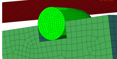
The final example is a hyperelastic/viscoelastic O-ring being compressed and then relaxed. The green circular component in the image above represents the O-ring. In a static step, the rigid plate compresses the O-ring into a groove in an elastic material. The plate is held fixed while the seal relaxes in a second step using the *VISCO procedure.

This model features include general contact, boundary conditions, and symmetry planes. When the analysis was run, the first step was not completed. The debugging process involves thoroughly examining partial results, animations, and the message file to identify the source of the problem.

The message file indicates that while the equilibrium is good, there are problems with contact. Note the messages about sticking and slipping.

The working hypothesis is that the O-ring is experiencing stick-slip behavior, which causes problems with the static procedure. A workaround is to use quasi-static implicit dynamics. In this case, switching the procedure makes things worse, which can happen. The message file indicates a contact problem with edge-to-face contact at nodes 4 and 4559, which are at the sharp edge of the groove.

Let us view the edges that are in the general contact. We can visualize GENERAL_CONTACT_EDGES_3 in the contact domain using Abaqus/Viewer. We notice that there are unwanted edges on the symmetry boundaries. There are options in general contact in Abaqus/Standard to remove edges from the contact domain. Let us remove those and try again.

Once the whole model is running, we can consider reverting to a static procedure. Making one change at a time works best so the procedure is not changed.

We are changing the contact to eliminate the edges on the symmetry plane and switch the first step to a dynamic procedure. This gives me physical time and a viscoelastic effect. It also offers us an inertial effect. This means we must pay close attention to the time for this step.

I am using a time of 0.1 for that step and a relaxation time of 30 seconds. Since the rate of loading for this small O-ring isn’t long compared to the relaxation time, 0.1 seems like a good time to use for that step.

Although step 1 is successful, the simulation fails yet again. We get past the compression step and into the VISCO step, but then it fails. By analyzing the partial results, animations, and the last saved result in step two, a deformation pattern is observed in the reduced integration mesh.

A plot of the seal’s deformed shape indicated the hourglassing of the C3D8RH elements. This is where perseverance is required. We can eliminate the reduced integration elements and put in fully integrated elements to eliminate the hourglassing effect. The next step is to switch the brick element to C3D8H and try again. Rerunning the simulation offers a complete result. The solution is now successful. We can work on model refinements at our leisure.

I decided to refine the mesh and round the edge of the groove. Often, convergence is more accessible to obtain when the edge is rounded. The radius of the round should be large enough to allow the mesh to conform to it. If you need a sharper edge, use a more refined mesh.

Once we implement these changes, the simulation is successful. This example has demonstrated the importance of persistence and adaptability in resolving convergence challenges.

General Debugging Techniques and Strategies for Finite Element Models

Debugging Abaqus/Standard convergence issues can be daunting. A checklist is crucial to identifying and resolving these challenges in your model.

Here are the key steps to keep in mind to effectively debug a model in Abaqus/Standard:

• Know your model features and how to use them properly.
• Identify the potential pitfalls that your model features can cause.
• Apply all available information to form a hypothesis.
  • Partial results are beneficial. Remember not to artificially limit the output while debugging.
  • Read the error/warning messages and analyze the message file.
• Define a workaround for the hypothetical problem.
• It isn’t uncommon for initial attempts to fail. Perseverance is the key to completing the analysis.

The last thing to remember is that through training and experience, one can understand the pitfalls of specific features. Training and experience allow users to sharpen their ability to hypothesize and implement practical solutions for convergence issues.

Here is a list of recommended training classes and resources for further learning.

• Obtaining a Convergence Solution with Abaqus
• Modeling Contact and Resolving Convergence Issues with Abaqus
• Abaqus/Explicit: Advanced Topics
• Buckling, Post Buckling, and Collapse Analysis with Abaqus
• Any training class is beneficial.

These educational resources are available on the SIMULIA website. I encourage you to explore these training opportunities if you are looking to enhance your problem-solving capabilities in debugging convergence issues with Abaqus/Standard.

Conclusion

In conclusion, debugging convergence issues in Abaqus/Standard is an intricate process that requires a deep understanding of the model’s features and potential problems. Training and experience assist in accurate hypothesis formulation to implement successful solutions. The Newton-Raphson method is central to the solver, and when non-convergence occurs, a systematic approach is employed to diagnose and remedy the issues.

Partial results, error messages, and animations are invaluable in this process and guide modifications to achieve successful outcomes. Persistence is required as initial attempts may only sometimes resolve the issues.

Eventually, a systematic and knowledgeable approach, backed by perseverance, is pivotal to mastering the debugging of finite element models in Abaqus/Standard.

To learn more about mastering debugging in Abaqus/Standard, we invite you to access our recorded session here.

---

Interested in the latest in simulation? Looking for advice and best practices? Want to discuss simulation with fellow users and Dassault Systèmes experts? The SIMULIA Community is the place to find the latest resources for SIMULIA software and to collaborate with other users. The key that unlocks the door of innovative thinking and knowledge building, the SIMULIA Community provides you with the tools you need to expand your knowledge, whenever and wherever.