Mastering Output Filtering in Abaqus/Explicit & Abaqus/Viewer

Key Takeaways

1. What is Output Filtering?
   Output filtering reduces unwanted noise in simulation data, highlighting relevant physical responses for better clarity and reliability.
2. The Problem of Aliasing:
   Aliasing occurs when data is sampled at a rate too low to capture high-frequency signals, leading to misleading results. The Nyquist frequency is a critical benchmark to avoid this issue.
3. Filtering Solutions in Abaqus:
   • Runtime Filters (Abaqus/Explicit): Prevent aliasing by filtering data before it is saved. The built-in anti-aliasing filter is highly effective.
   • Post-Processing Filters (Abaqus/Viewer): Allow further refinement and smoothing of data after simulation.
4. Best Practices for Output Filtering:
   • Perform a frequency analysis to identify significant dynamic characteristics.
   • Use the 6x rule of thumb for output sampling rates to ensure data fidelity.
   • Avoid over-filtering, which can remove meaningful structural responses.
   • Monitor extreme values efficiently using runtime filter operations like MAX or ABSMAX.
5. Mitigating Filter Artifacts:
   Be aware of time shifts and end distortions caused by filtering, and design simulations to minimize their impact.
6. A Robust Workflow:
   Combine frequency analysis, runtime filtering, and post-processing to ensure clean, interpretable data for critical engineering decisions.

What is Output Filtering?

Output filtering is the process of applying mathematical techniques to simulation results to reduce unwanted noise and highlight the relevant physical responses of a system. By filtering simulation outputs, engineers can improve the clarity and reliability of their data, making it easier to interpret true system behavior and draw accurate conclusions.

Introduction

In finite element analysis, particularly with dynamic explicit simulations, the data generated can be vast and complex. A common challenge engineers face is distinguishing the true structural response from high-frequency solution noise. Raw data from Abaqus/Explicit can be filled with oscillations that, while mathematically part of the solution, can obscure the underlying physical behavior of the model. This is where output filtering becomes an indispensable tool. The proper application of filters enables analysts to attenuate this noise, prevent significant data misinterpretation, and gain a clear, actionable understanding of a model’s dynamic performance.

This blog offers an in-depth exploration of the technical principles and practical applications of output filtering in both Abaqus/Explicit and Abaqus/Viewer. We will explore the fundamental problem of aliasing, detail the extensive filtering options available, and provide robust guidance for configuring simulations to yield clean, reliable, and insightful data.

The Peril of Aliasing: When Data Deceives

At its core, aliasing is a form of data corruption caused by an inadequate output frequency. Imagine trying to understand a fast-spinning wheel by only looking at it once every second. Depending on when you glance, the wheel might appear stationary, spinning slowly, or even rotating backward. You are sampling reality at a rate too slow to capture the true motion. In Simulation, the same phenomenon occurs.

The Nyquist-Shannon sampling theorem provides the mathematical foundation for this concept.

It states that to accurately reconstruct a signal, the sampling frequency must be at least twice the highest frequency component present in that signal. This threshold, known as the Nyquist frequency, is a critical benchmark in data acquisition.

When you request simulation output at a rate below this, you risk aliasing. The data points you save are individually correct and lie on the true, high-frequency curve, but when plotted, they create a new, misleading waveform that doesn’t exist in reality.

Visualizing Aliasing: From Zoetropes to Turbines

A classic, intuitive example of aliasing is the zoetrope. This 19th-century device creates the illusion of motion from a sequence of static images. In a modern simulation context, consider a rapidly rotating rigid body animated with a specific frame rate. Due to the relationship between the spin rate and the output rate, the object can appear to deform and flex as if it were made of a soft material. This “frame rate effect” is a direct visual manifestation of aliasing, leading to a complete misinterpretation of the object’s rigid body motion.

A more direct engineering example involves simulating a turbine fan where a blade detaches and strikes the outer casing. When the animation frames are saved too infrequently, the fan can appear to rotate backward. An analyst unfamiliar with aliasing might waste valuable time investigating a non-existent problem with their boundary conditions, believing the prescribed rotation was not enforced correctly. The issue isn’t the physics simulation; it’s the way it’s observed. To see the true counter-clockwise rotation, more frames must be saved, capturing the fan’s position at smaller increments of its revolution.

Aliasing in XY Plots: A Cantilever Beam Case Study

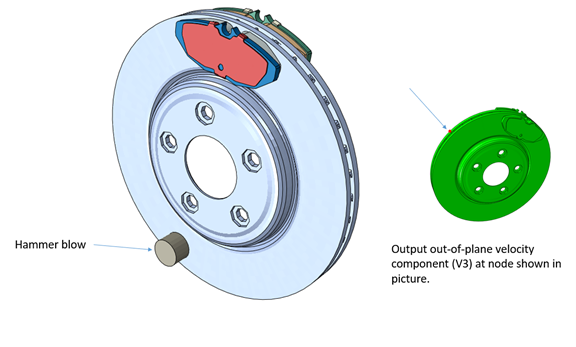
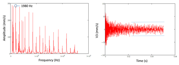
The impact of aliasing is just as profound on time history plots. Consider a simple cantilever beam subjected to a suddenly released pressure load, causing it to vibrate freely.

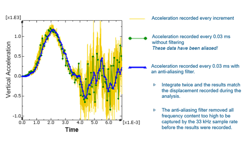
• The “True” Signal: If we record the vertical velocity at the beam’s tip at every single time increment of the Abaqus/Explicit simulation, we obtain a clean, high-resolution curve that accurately depicts the vibrational motion. This represents the ground truth.
• The Aliased Signal: Now, if we request the same output variable but at a much lower frequency (e.g., every few hundred increments), the resulting plot is drastically different. The handful of data points we collect fall on the true curve, but they miss all the intervening peaks and troughs. Connecting these points creates a new, lower-frequency signal that completely misrepresents the beam’s behavior.

In a simple case like this, we have the luxury of the high-resolution data for comparison. In a complex, real-world analysis, we often only have the low-frequency data. Without an understanding of aliasing, an engineer might mistakenly conclude the structure’s vibrational response is much slower and has a lower amplitude than it actually does, leading to flawed design decisions.

Which Results Are Most Susceptible to Aliasing?

Not all output variables are created equal when it comes to aliasing. The susceptibility is directly related to the variable’s “frequency content.” Operations that involve integration tend to smooth out a signal, removing high-frequency components. Conversely, operations involving differentiation tend to amplify them.

This leads to a clear spectrum of susceptibility in structural analysis:

• Low Susceptibility (Displacements): Displacement is the result of integrating velocity over time, which itself is the integral of acceleration. This double integration process naturally filters out high-frequency noise. As a result, displacement plots are often smooth and less prone to aliasing issues.
• Medium Susceptibility (Velocities): As the first integral of acceleration, velocity contains more frequency content than displacement but is generally less noisy than acceleration. It occupies a middle ground.
• High Susceptibility (Accelerations and Reaction Forces): These quantities are often the “rawest” signals in an explicit dynamic analysis. They directly reflect the high-frequency waves propagating through the mesh elements and are therefore extremely noisy and highly susceptible to aliasing.

Quasi-static simulations, despite being run in Abaqus/Explicit, typically have very slow loading rates, which minimize dynamic effects and render aliasing a non-issue. However, for any analysis involving impacts, collisions, or high-frequency vibrations, careful consideration of output requests for acceleration and force is paramount.

A Two-Pronged Solution: Filtering in Abaqus/Explicit and Abaqus/Viewer

Abaqus provides a comprehensive suite of filtering tools to combat noise and aliasing. These tools can be deployed at two distinct stages: during the simulation run (runtime filtering) and after the simulation is complete (post-processing).

1. Runtime Filtering in Abaqus/Explicit

Runtime filters are the first and most critical line of defense. They operate on the data before it is written to the output database (ODB) file. This approach is fundamentally important because once a signal is undersampled and the aliased data is saved to the ODB, the lost high-frequency information cannot be recovered.

Abaqus/Explicit offers several industry-standard filter types that you can define using the *FILTER keyword:

• Butterworth: Known for its maximally flat frequency response in the passband, making it a very popular general-purpose filter.
• Chebyshev Type I: Exhibits a steeper roll-off than a Butterworth filter, but at the cost of introducing ripples in the passband.
• Chebyshev Type II: Has ripples in the stopband instead of the passband.

The Built-In Anti-Aliasing Filter: Your Default Choice

For most applications, defining a custom filter is unnecessary. Abaqus provides a robust, pre-configured anti-aliasing filter that is highly effective. When you request this filter, Abaqus automatically implements a second-order, low-pass Butterworth filter. The intelligence is in how it sets the cutoff frequency.

The cutoff frequency is automatically defined as one-sixth (1/6) of the output sampling rate you specify in your output request.

Let’s break this down with an example. Suppose you request history output every 0.1667 milliseconds.

1. Output Sample Rate: 1 / (0.1667 x 10⁻³ s) = 6,000 Hz (6 kHz).
2. Nyquist Frequency: Per the sampling theorem, the highest frequency you can possibly resolve is half the sample rate, which is 3 kHz. Any frequency content above 3 kHz in your raw signal risks causing aliasing.
3. Filter Cutoff Frequency: The anti-aliasing filter sets its cutoff at 1/6th of the sample rate: 6,000 Hz / 6 = 1,000 Hz (1 kHz).

By setting a cutoff at 1 kHz, the filter strongly attenuates all frequencies above this, ensuring that any content near the problematic 3 kHz Nyquist frequency is eliminated before the signal is sampled and written to the ODB. This provides a clean, unaliased representation of the signal. A significant benefit of using this filter is that Abaqus will issue a warning if your chosen output rate is too low for the filter to be effective, acting as a built-in safety check against aliasing.

2. Post-Processing Filters in Abaqus/Viewer

If you have successfully saved a rich, high-frequency signal to the ODB (ideally using a runtime filter), you can perform additional filtering within Abaqus/Viewer. This is done through the Operate on XY data dialog box. Post-processing is useful for:

• Comparing different filter types and cutoff frequencies without re-running the analysis.
• Applying smoothing for presentation purposes.
• Further reducing noise that was not fully eliminated at runtime.

A Key Difference: Single-Pass vs. Dual-Pass Filtering

A crucial technical distinction exists between runtime and post-processing filters.

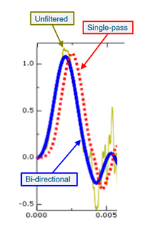
• Abaqus/Explicit Runtime Filters: These are single-pass, causal filters. They process data only in the forward direction of time, as the simulation progresses. This is a physical necessity—the solver cannot “see into the future” to know what data is coming. A consequence of this single-pass operation is a phase shift, or time delay, in the filtered output. The peaks of the filtered curve will be shifted slightly to the right (later in time) compared to the raw signal.
• Abaqus/Viewer Filters: These are dual-pass (or bidirectional) filters. They process the entire data series forward and backward in time. The backward pass effectively corrects the phase shift introduced by the forward pass. As a result, Viewer-filtered signals are perfectly aligned in time with the original unfiltered signal.

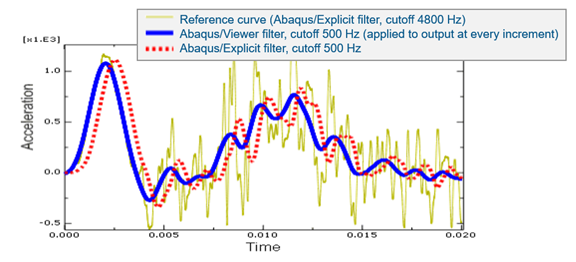
While often small, this time shift induced by runtime filters is a real distortion that analysts should be aware of, especially when trying to precisely correlate events in time.

Best Practices

Theory is valuable, but effective filtering requires a practical approach. The goal is to balance data fidelity with manageable file sizes.

·        How to Choose Your Output Frequency

The ideal output frequency is high enough to capture the structurally significant response but not so high as to generate unmanageably large ODB files. A systematic approach is best:

1. Perform a Natural Frequency Analysis: Before running your explicit dynamic simulation, run a natural frequency extraction analysis (*FREQUENCY) in Abaqus/Standard on the same model. This will tell you the characteristic frequencies of your structure’s dominant vibration modes.
2. Identify the Highest Structurally Significant Frequency: Your structure may have hundreds of modes, but typically only the first several are structurally significant. Identify the highest-frequency aspect of your engineering problem that you genuinely care about. For many structural vibration problems, this range is between 50 Hz and 5,000 Hz. This is usually much, much lower than the highest frequency in the entire model, which governs the stable time increment (often in the hundreds of kilohertz).
3. Design Your Output Rate: Use the highest significant frequency to determine your output rate. A good rule of thumb is to set a filter cutoff frequency at or slightly above this value. If you use the built-in anti-aliasing filter, you can work backward:

• Desired Cutoff Frequency: Let’s say 5,000 Hz.
• Required Output Sample Rate: This must be 6 times the cutoff, so 6 * 5,000 Hz = 30,000 Hz.
• Required Output Time Interval: 1 / 30,000 Hz ≈ 3.33 x 10⁻⁵ seconds (0.0333 ms).

Requesting history output at this interval with the anti-aliasing filter provides a robust starting point. It’s often pragmatic to increase this sampling rate (e.g., by a factor of 2) if disk space allows. It is always better to have too much data than not enough.

·        The Danger of Over-Filtering

Just as undersampling is problematic, so is over-filtering. If you set your filter cutoff frequency too low, you can inadvertently remove physically meaningful parts of your structural response.

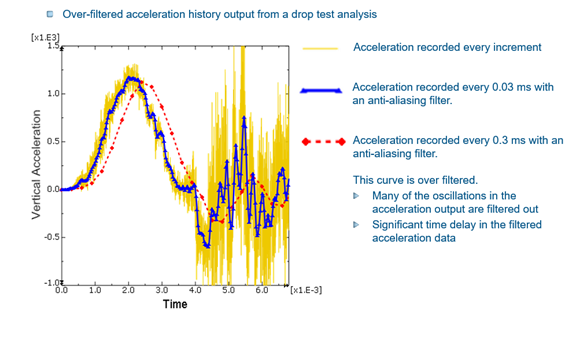
Revisiting the example of the noisy acceleration signal, if we apply a filter with a very low cutoff, the resulting curve might look smooth and clean, but it will have filtered out the entire structural vibration signature. The over-filtered signal might have a drastically reduced peak amplitude and a significant time shift, making it look more like the response of a heavily damped, single-degree-of-freedom system than a complex structural vibration. This is another form of misinterpretation.

·        Advanced Technique: Monitoring for Extreme Values

A powerful and often underutilized feature of runtime filters is the ability to monitor for extreme values. By adding the OPERATION parameter to your *FILTER or *OUTPUT definition, you can track peaks without saving the entire time history.

OPERATION = MAX: Reports the maximum value encountered up to that point in time.
OPERATION = MIN: Reports the minimum value.
OPERATION = ABSMAX: Reports the maximum absolute value.

This is exceptionally useful for field output. Imagine trying to find the maximum principal strain in a large model during a crash event. Instead of saving contour plots for thousands of time increments, you can request field output for the strain variable with OPERATION = MAX at a single time point (the end of the step). The resulting contour plot will show, for each element, the peak value it experienced during the entire simulation. Abaqus also writes the time at which this peak occurred to the results file, allowing you to efficiently identify the most critical moment for further detailed analysis.

·        Mitigating Inherent Filter Distortions

Filters are powerful but not perfect. Beyond the time shift discussed earlier, another artifact to be aware of is end distortion.

Filtering algorithms require a certain window of data points to perform their calculations. At the very beginning and very end of a signal, this window is incomplete. This can lead to distortions or “ringing” in the filtered output near the start and end times. If you have a critical event of interest that happens right at the end of your simulation step, the filtered representation of that event may be compromised by end distortion. A simple solution is to extend the simulation time so the event of interest occurs well within the analysis period, away from the endpoints.

Conclusion

Output filtering is not an optional extra; it is a fundamental component of sound engineering practice in explicit dynamics. By mastering these tools, you can move from noisy, ambiguous data to clear, interpretable results.

A robust workflow is key:

1. Understand Your Structure: Use a frequency analysis to determine the significant dynamic characteristics of your model.
2. Filter at the Source: Always use runtime filters in Abaqus Explicit to create a rich, unaliased ODB file. The built-in anti-aliasing filter is the recommended starting point for its simplicity and effectiveness.
3. Choose Output Rates Wisely: Base your output frequency on your desired structural response, using the 6x rule of thumb for the anti-aliasing filter. When in doubt, save more data.
4. Leverage Post-Processing: Use the bidirectional filters in Abaqus/Viewer for additional smoothing and comparative analysis, confident that your underlying data is sound.
5. Be Aware of Artifacts: Understand the effects of time shifts and end distortions and design your simulations to minimize their impact on your interpretation.

By adopting this methodical approach, engineers can confidently navigate the complexities of dynamic data, ensuring their simulation results provide a solid, accurate foundation for critical design decisions. To learn more about output filtering, check out our webinar here.

Extending Output Filtering Workflows on the 3DEXPERIENCE Platform

Within the 3DEXPERIENCE platform, output filtering workflows in Abaqus can be managed as part of a model-based, data-centric simulation environment. Rather than treating filtering as an isolated solver or Viewer operation, the platform enables it to be included within a traceable simulation lifecycle.

Abaqus analyses executed through SIMULIA roles (such as Physics Simulation or Structural Simulation Engineer) retain filtering definitions, including *FILTER parameters, output requests, and sampling rates, within the simulation object or associated input data. This ensures that:

• Filter configurations are persistent and version-controlled: Changes to cutoff frequencies, anti-aliasing settings, and output intervals are tracked alongside model revisions.
• Simulation provenance is maintained: Results can be correlated with the input configuration used to generate them.
• Simulation data is centrally managed: Large datasets generated with high sampling rates are stored and governed within the platform environment, improving accessibility and reducing duplication.

Post-processing operations typically performed in Abaqus/Viewer, including XY data filtering and signal conditioning, can be reproduced through scripting or process automation workflows where required. This supports:

• Standardization of filtering methodologies across teams.
• Automation of result extraction, including filtered signals and extreme value monitoring (e.g., MAX/ABSMAX operations), when implemented through user-defined processes.
• Reuse of simulation processes, improving consistency across programs.

By incorporating output filtering within a governed data environment, the 3DEXPERIENCE Platform supports more consistent handling of aliasing and signal fidelity, while maintaining traceability of how simulation results are generated and interpreted.

Interested in the latest in simulation? Looking for advice and best practices? Want to discuss simulation with fellow users and Dassault Systèmes experts? The SIMULIA Community is the place to find the latest resources for SIMULIA software and to collaborate with other users. The key that unlocks the door of innovative thinking and knowledge building, the SIMULIA Community provides you with the tools you need to expand your knowledge, whenever and wherever.